Introduction
To understand transformers, you must understand attention. Many explanations focus on the how rather than the why, making terms like queries, keys, and the underlying math feel arbitrary. You can memorize the attention formula and still have no idea why it actually works. But once you grasp the core intuition behind each step, attention becomes easy to remember and reason about.
In this article, we’ll explore both the how and the why. Specifically, we will look at:
- The role and intuition behind queries, keys, and values.
- Why we “scale” in scaled dot-product attention.
This article focuses on single-head attention. Its extension, multi-head attention, will be covered in a follow-up piece.
Note: English is not my native language, so I used AI for proofreading and polish. The concepts and explanations are entirely my own.
Attention
Vaswani et al. [1] established modern attention as the core of the transformer architecture. While attention itself was not new (see [2]), their variant—Scaled Dot-Product Self-Attention—changed how models process text. Prior architectures like RNNs and LSTMs processed text sequentially word by word, creating two critical bottlenecks:
- No parallelization: Step-by-step processing slowed down training.
- Vanishing long-range context: Connecting distant words (e.g., a subject at the start of a long sentence to a verb 20 words later) was difficult.
Self-attention eliminated these bottlenecks by allowing every token (a word or sub-word unit) to directly attend to every other token in a single operation. This direct connection enabled massive parallelization and solved context loss, paving the way for modern large-scale models.
In this article, we will examine the self-attention mechanism as presented in the original paper. A basic familiarity with vector embeddings, elementary Python, and linear algebra fundamentals—specifically matrix multiplication and dot products—will help, though key concepts are explained along the way.
What problem does attention solve? A conceptual overview
Let’s first clarify the problem we want to solve.
Understanding language is hard, partly because the meaning of a word depends on its context. Take these two sentences:
- “You should duck when the ceiling is low.”
- “The hunter saw a duck in the pond.”
In the first sentence, “duck” functions as a verb (duck: action), which we deduce because it appears alongside “ceiling” and “low.” The second sentence refers to the animal (duck: animal), which we infer from “hunter” and because the duck is the direct object being “seen.” You can’t physically see a verb.
This context dependency posed a major challenge for natural language processing (NLP). But before tackling context, researchers had to solve an even more fundamental issue: how to represent words so computers could process them at all. Solving this was an incremental process, evolving from one-hot encodings to count-based approaches and eventually generative methods ([3], [4]) like Word2Vec [5]. The unifying idea was mapping each word to a vector of numbers—a word embedding. A word embedding captures semantic meaning, placing words with similar meanings close together in vector space. For example, the embeddings for “man” and “boy” should be close to each other, but far from an unrelated word like “banana.”
The text processing pipeline works roughly as follows:
Tokenization: A sequence of text is split into pieces (words, subwords, or characters), and each unique piece is assigned a numerical identifier called a token. (For simplicity in this text we’ll assume that one word is mapped to a token.) In frameworks like Hugging Face, the
AutoTokenizerclass handles this step.Embedding Lookup: Each token is mapped to a vector, historically using pre-trained lookup tables like Word2Vec or GloVe [6]. Today, models typically start with randomly initialized embeddings that are learned end-to-end during training.
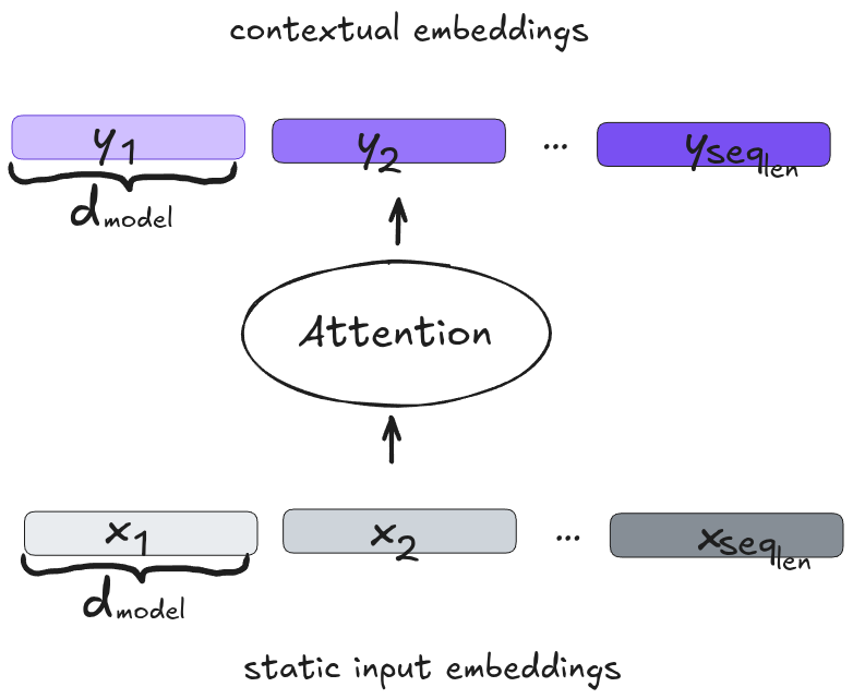
The important point here is that regardless of how these embeddings are initialized, the same token always maps to the same vector. Because of this, we call them static embeddings. Static embeddings are completely oblivious to context. They provide a solid baseline representation of a word’s default meaning, but they must be refined to fit the sentence they appear in. And this is precisely what the attention mechanism solves: it takes static embeddings as input and updates them into contextual embeddings based on the surrounding tokens. This transformation is illustrated in Figure 1. Notice that the input and output vectors share the same dimensionality (\(d_{\text{model}}\)), while \(seq_{\text{len}}\) denotes the number of tokens processed together.
To see how contextual embeddings are computed, we can break the mechanism down into three core ideas:
- Vector Transformations: Embeddings are vectors and vectors can be transformed into other vectors via matrix multiplication.
- Weighted Averaging: To incorporate context, attention uses a form of weighted averaging. This was originally introduced via a database analogy. This analogy is where the terms queries, keys, and values originate: in a traditional database, you send a query to match an exact key and retrieve its associated value. Attention extends this by replacing exact matching with soft matching. Every key receives a relevance score relative to the query, yielding a weighted sum of all values. (Statisticians will recognize this as a vector-valued generalization of Nadaraya-Watson kernel regression; see [7], [8].)
- Learned Projections: Queries, keys, and values are vectors generated by multiplying static input embeddings by three projection matrices. Learning these matrices during training is how the transformer adapts to language.
Let’s examine each of these ideas in detail.
Embeddings are vectors
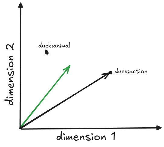
It might sound trivial, but this is a fundamental concept to keep in mind: embeddings are vectors. As such, they point to specific positions in an \(n\)-dimensional space (see Figure 2).
Consider an ambiguous word whose meaning depends on context—like “duck” from our previous example. It is helpful to think of the initial, static embedding of “duck” as a baseline vector that lies somewhere between its possible specific meanings. This idea is visualized in Figure 2, where the static vector for “duck” is shown in green, alongside the target vectors for duck:animal and duck:action.
If we encounter a sentence where the context demands the “action” meaning, the attention mechanism must do two things: 1. Identify the target: Determine from the surrounding tokens that we need to head toward duck:action (the black vector). 2. Apply the transformation: Shift the green static vector to its new, contextual position in space.
Now, how can a model transform the static embedding into a contextualized version when it doesn’t even know what that final version should look like? This seems like an impossible task.
To see how this works, let’s take a quick step back to review the core idea of neural networks and how they are trained. (Feel free to skip the next section if you are already familiar with the basics.)
A quick review on neural network training
Remember that the attention mechanism is a core component of the transformer—a neural network composed of layers with trainable parameters.
The central premise of neural networks is that an optimal set of parameter values exists to produce our desired output. In image classification, for example, we input images and expect correct labels. Initially, random parameters yield poor predictions. Training is the process of discovering parameters that make those predictions accurate. Crucially, we never calculate these ideal values explicitly. Instead, we frame learning as an optimization problem. We measure performance using a loss function—which quantifies how far our predictions are from the correct answers. Minimizing this loss directly yields a well-performing model. Optimization algorithms (typically variants of gradient descent) dictate how to adjust parameters at each step to steadily reduce error. We repeat this process across many examples until performance stabilizes.
The key takeaway: we don’t manually program the parameters. Instead, we define the architecture, the loss function, and the optimization method—and the model learns the ideal parameters through training.
With this reminder in place, we can return to our original question.
How can the model transform a static embedding into its contextualized version without knowing that version beforehand?
The short answer: The transformation that “finds” the right contextual embedding is learned.
To understand this, recall that our goal is to map an input vector to a specific output vector. Mathematically, this is a linear transformation: we multiply the input vector by a matrix (see Figure 3).
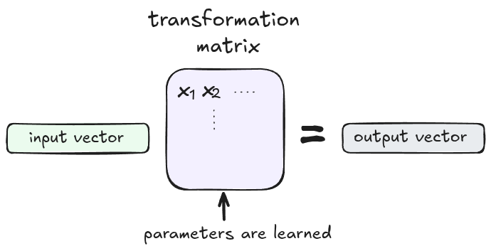
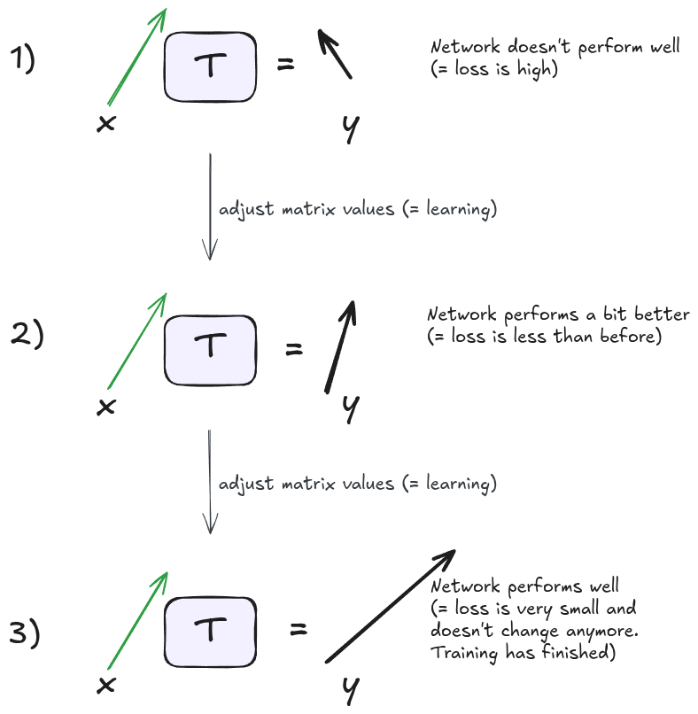
Initially, this matrix is filled with random values, producing poor, unhelpful embeddings that lead to a high loss (see Figure 4, top row). During training, the optimization algorithm continuously nudges these parameters toward values that minimize the loss (see Figure 4, middle row).
Crucially, the matrix entries are what we actually learn. Once training concludes and the transformer achieves high performance, the matrix has successfully encoded the exact transformation required. We discover both the transformation and the final embeddings without ever having to explicitly define or know those target embeddings beforehand (see Figure 4, bottom row).
This is the foundational principle behind contextual embeddings. However, a single standard linear transformation isn’t enough to capture complex language relationships. To truly incorporate context, the attention mechanism uses not just one, but several interacting matrices, each playing a distinct role. That is what we will explore next.
How do we take context into account?
Our goal is to understand how the meaning of a word is shaped by its surrounding words—its context. Every word in the sequence contributes to creating the final contextual embedding, i.e. every word in the sequence is part of the context. The core idea of attention is: each contextual embedding is a weighted sum of all static input embeddings. The weights reflect how relevant each surrounding word (represented by its static input embedding) is to the target word for which we want to compute the contextual embedding. As already mentioned, if you are familiar with non-parametric statistics, you can view this as an instance of Nadaraya-Watson kernel regression (see [7]). If not, don’t worry – the following database analogy is an intuitive way to picture it.
The database analogy
Imagine a simple database of colors, which we can represent as a Dictionary in Python as follows:
Code
import numpy as np

database = {
    'Red':    np.array([255, 0,   0  ]),
    'Blue':   np.array([0,   0,   255]),
    'Yellow': np.array([255, 255, 0  ]),
    'Green':  np.array([0,   128, 0  ])
}
The keys are color names and the values are their RGB vectors. If you query the database for an exact key, like database['Red'], you get [255, 0, 0]. This is equivalent to a weighted sum where the weight for ‘Red’ is 1 and all others are 0.
But what if the query were something more abstract? For example: “What is the color of a sunset?” There is no exact match for that in our database. Instead, we match the keys against this query in a “soft,” probabilistic way. Imagine the keys as individuals scoring their own relevance to the question:
‘Red’ says: “A sunset contains a large part of me.” It claims a high relevance weight of 0.6.
‘Yellow’ feels relevant but a bit less so, responding with 0.3.
‘Blue’ senses a faint connection at twilight, giving a 0.1.
‘Green’ bows out entirely with a 0.0.
This gives a clean set of weights that are between 0 and 1 and sum to 1:
| Key | Attention Weight |
|---|---|
| Red | 0.6 |
| Yellow | 0.3 |
| Blue | 0.1 |
| Green | 0.0 |
In deep learning literature, these are called attention weights. They dictate exactly how much attention to pay to each key.
The final result of our query is a weighted sum of the color vectors:
Code
result = 0.6*database['Red'] + 0.3*database['Yellow'] + 0.1*database['Blue'] \
 + 0.0*database['Green']
print(result) # = [229.5  76.5  25.5], a warm orange-red
[229.5 76.5 25.5]This might seem like a silly example, but it captures exactly the idea behind attention: the result is not a single retrieved item, but a sum of all values, weighted by their relevance to the query. This is how context gets taken into account — the more relevant a key within the sequence is to the query, the more its value contributes to the final result. And that final result is, of course, the contextual embedding.
Now that we have the intuition down, the remaining question is practical: how do we actually calculate these weights mathematically, and where do the queries and keys come from? That is what we will look at next.
How to compute the attention weights for a single query?
Computing attention weights is straightforward — if queries, keys, and values are vectors.
Imagine a query \(\mathbf{q}\) is not a sentence in human language, but a vector of numbers the computer can work with directly. The same goes for a key, \(\mathbf{k}\). To compute how relevant \(\mathbf{k}\) is to \(\mathbf{q}\), we can compute the inner (dot) product of the two vectors – a standard way to measure similarity between vectors. The more similar two vectors are, the larger their dot product. We allow ourselves some liberty here and interpret this similarity as “relevance” of the key to the query.
Because \(\mathbf{q}\) and \(\mathbf{k}\) are row vectors, their inner product is simply \(\mathbf{q}\mathbf{k}^T = z\), where \(z\) is a scalar representing relevance. (Note that I assume here that the query and key vectors are row vectors. This is just a convention, we could also use column vectors, but we would need to adjust the formulae accordingly. Column vectors are more common in the math and ML literature, but when programming we usually need to convert them to row vectors due to how vectors are efficiently stored in computer memory. Therefore, I thought we might as well use row vectors to start with.)
How to apply this to embeddings?
Recall from Figure 1 that we have several static embeddings of which we want to compute contextualized versions. We denoted the number of static input embeddings that are processed together as one sequence as \(seq_{\text{len}}\). Now imagine that for each static embedding \(\mathbf{x}_i\), a magical process creates three distinct vectors: a query \(\mathbf{q}_i\), a key \(\mathbf{k}_i\), and a value \(\mathbf{v}_i\) as visualized in Figure 5. (More on that in Section 8)
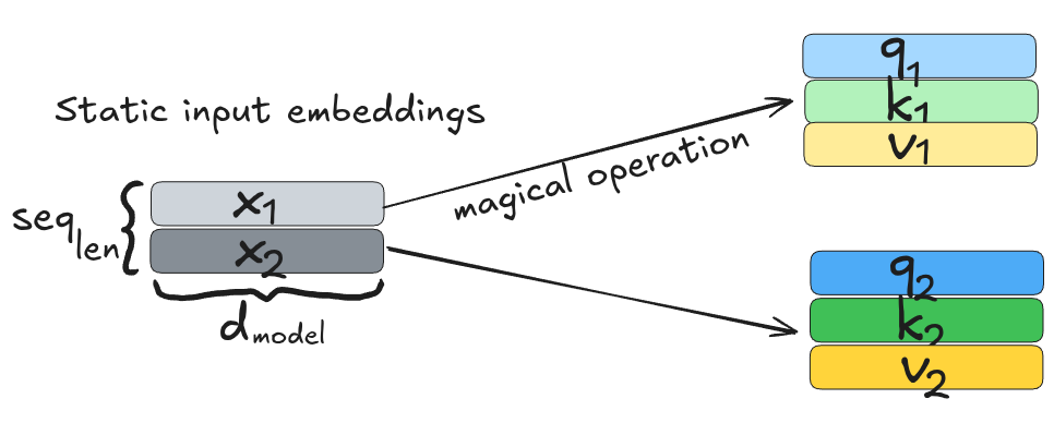
We can interpret this as a database with two entries: database={\(\mathbf{k}_1\):\(\mathbf{v}_1\), \(\mathbf{k}_2\):\(\mathbf{v}_2\)}. We also have two queries, \(\mathbf{q}_1\) and \(\mathbf{q}_2\). Now, as explained, to compute how relevant the database entries are with respect to each query we compute the dot products between a query and each key. Thus, we use the dot product as similarity function. Concretely, to compute how relevant each key is for \(\mathbf{q}_1\) in our example, we compute the dot products \(\mathbf{q}_1 \mathbf{k}_1^T\) and \(\mathbf{q}_1 \mathbf{k}_2^T\). The results are two weights which we can collect in a vector \(\mathbf{z}_1\). Furthermore, if we stack all key row vectors into a matrix \(\mathbf{K}\), we can compute the relevance scores for \(\mathbf{q}_1\) against all keys at once using a vector-matrix product:
\[ \mathbf{z}_1 = \mathbf{q}_1 \mathbf{K}^T \]
And here is a visual for a better mental picture:
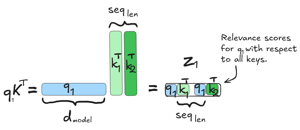
These unnormalized entries in the vector \(\mathbf{z}_1\) are often referred to as scores. We have established that each individual score is a dot product of two vectors and the vectors are of dimension \(d_{\text{model}}\). This means that for each score we had to add \(d_{\text{model}}\) products together. The larger \(d_{\text{model}}\) the more numbers we add together the larger the score. But we don’t want very large scores as they can negatively affect the model training, thus we need to keep their values in check. This can be achieved by normalizing each score by dividing it by the square root of the vector dimension \(d_{\text{model}}\), thus, \(\mathbf{z}_1 / \sqrt{d_{\text{model}}}\). More on this in the optional chapter Why scaling.
Also, recall from the preceding discussion that we want the attention weights for a query to sum to one. We can achieve this by passing the normalized scores vector through the softmax function. The result of this – finally – are the attention weights \(\boldsymbol{\alpha}_1\):
\[ \boldsymbol{\alpha}_1 = \text{softmax}\left(\dfrac{\mathbf{z}_1}{\sqrt{d_{\text{model}}}}\right) \]
Note that \(\boldsymbol{\alpha}_1\) is a vector that contains all the attention weights for \(\mathbf{q}_1\) with respect to all keys in the database. The sum of all entries is 1.
Why scaling?
As a reminder: we are looking at single-head scaled dot-product attention. Here is where the term scaled comes from. We must divide the vector \(\mathbf{z}_1\) by \(\sqrt{d_{\text{model}}}\), the square root of the query vector’s dimension. To see why we need it, consider what happens when the query and key vectors have many dimensions, thus \(d_{\text{model}}\) is a large number. The dot product \(\mathbf{q}_1 \cdot \mathbf{k}_i\) sums \(d_{\text{model}}\) individual products \(q_{1,j} k_{i,j}\). If we assume each component of \(\mathbf{q}_1\) and \(\mathbf{k}_i\) is independent, zero-mean, and unit-variance, then each individual product \(q_{1,j} k_{i,j}\) also has variance 1 – but the dot product itself, being a sum of \(d_{\text{model}}\) such independent terms, has variance \[ \text{Var}(\mathbf{q}_1 \cdot \mathbf{k}_i) = \sum_{j=1}^{d_{\text{model}}} \text{Var}(q_{1,j} k_{i,j}) = d_{\text{model}}. \] In practice, this means the scores in \(\mathbf{z}_1\) become more spread out as \(d_{\text{model}}\) grows — even when no key is genuinely more relevant than another, some scores will land noticeably higher than others purely by chance.
This is a problem for softmax, since it’s an exponential function: even a modest gap between the largest score and the rest gets amplified dramatically. The result is that softmax becomes overconfident, pushing nearly all the weight onto a single key and squeezing the rest toward zero — a phenomenon called saturation. Saturated softmax outputs have tiny gradients almost everywhere, which slows down or stalls learning. (You can refer to this post if you need to brush up on the derivative of the softmax function.)
Dividing every score by \(\sqrt{d_{\text{model}}}\) fixes this: since the variance of the scores grows with \(d_{\text{model}}\), dividing by \(\sqrt{d_{\text{model}}}\) brings it back down to a constant, regardless of dimensionality — keeping softmax’s input in a well-behaved range no matter how large \(d_{\text{model}}\) is.
How to compute the attention weights for all queries using matrix notation?
Thus far we have computed the attention weights for a single query. Note that with a tiny change in our computation we can compute the attention weights for all queries in one go. For that we simply collect all query vectors in a matrix \(\mathbf{Q}\) as shown the figure below. The output is the matrix \(\mathbf{Z}\) with each row i being the relevance scores for query i.
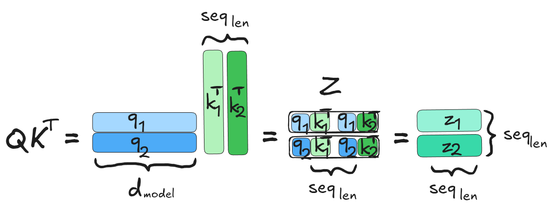
Again, to compute the attention weights we need to normalize the scores and pass each row through softmax (row-wise softmax). This can now be compactly written as:
\[ \mathbf{A} = \text{softmax}\left(\frac{\mathbf{QK}^T }{ \sqrt{d_{\text{model}}}}\right) \] Thus now \(\mathbf{A}\) is the matrix with each row \(\boldsymbol{\alpha}_i\) being the attention weights for query i.
Scaled dot-product attention (Single-Head)
As mentioned in the introduction, we start with the simpler single-head version first. Once we master how it works, scaling up to multi-head attention will be easy.
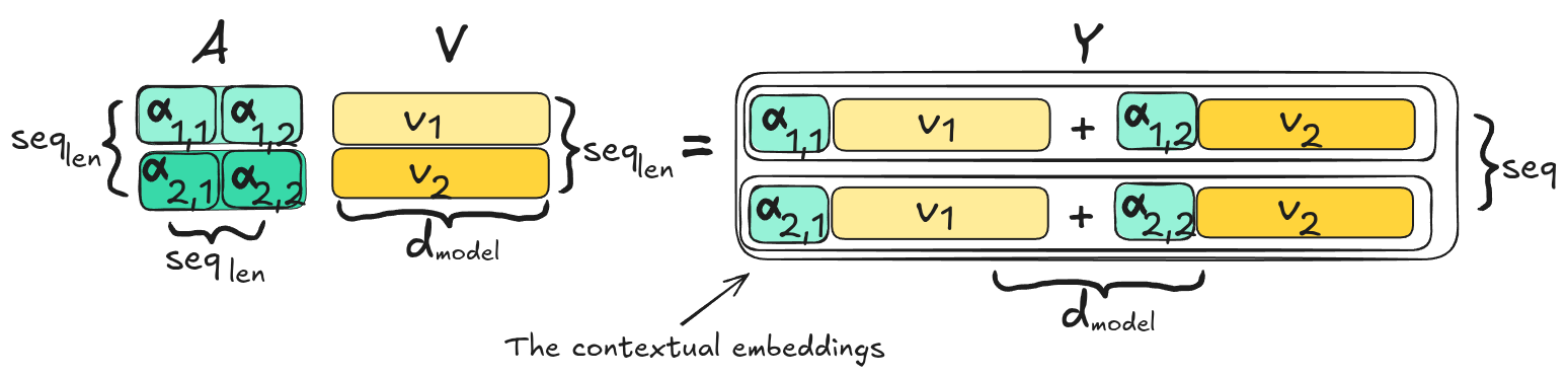
Now that we can compute the attention weights, we are ready to compute the contextual embeddings—which is our ultimate goal. Recall from our database example that a contextual embedding is the weighted sum of the values of each database entry, with the weights being the attention weights.
In our setup, this means the contextual embedding for the static input embedding \(\mathbf{x}_1\) is the weighted sum of the value vectors \(\mathbf{v}_1\) and \(\mathbf{v}_2\), weighted by the entries in the vector \(\boldsymbol{\alpha}_1\).
Thus, the contextual embedding \(\mathbf{y}_1\) is simply: \[ \mathbf{y}_1 = \alpha_{1,1} \mathbf{v}_1 + \alpha_{1,2} \mathbf{v}_2 \] where \(\alpha_{1,1}\) denotes the first component of \(\boldsymbol{\alpha}_1\) and \(\alpha_{1,2}\) the second.
Again, we can collect the row vectors \(\mathbf{v}_i\) into a matrix \(\mathbf{V}\) and write the sum above as a vector-matrix product: \[ \mathbf{y}_1 = \boldsymbol{\alpha}_1 \mathbf{V}, \qquad \boldsymbol{\alpha}_1 \in \mathbb{R}^{1 \times seq_{\text{len}}}, \quad \mathbf{V} \in \mathbb{R}^{seq_{\text{len}} \times d_{\text{model}}} \]
The result \(\mathbf{y}_1 \in \mathbb{R}^{1 \times d_{\text{model}}}\) is a vector of the exact same dimension as the static input embedding it replaces—just now enriched with context. That’s our contextual embedding!
Analogous to what we’ve done before, we can collect all weight vectors \(\boldsymbol{\alpha}_i\) into the matrix \(\mathbf{A}\). The product \(\mathbf{AV}\) then gives all contextual embeddings \(\mathbf{Y}\) in one go. This is visualized below for two database entries:
Putting it all together gives us the exact scaled dot-product attention formula from Vaswani et al.:
\[ \text{Attention}(\mathbf{Q}, \mathbf{K}, \mathbf{V}) = \mathbf{AV} = \text{softmax}\left(\frac{\mathbf{Q}\mathbf{K}^T}{\sqrt{d_{\text{model}}}}\right)\mathbf{V} \]
That’s it! Take a moment to pat yourself on the back—we’ve just covered the core mechanics of attention and as such the heart of the transformer architecture.
We aren’t quite done yet, though. Two remaining questions stand in our way:
- Where do these vectors \(\mathbf{q}_i\), \(\mathbf{k}_i\), and \(\mathbf{v}_i\) actually come from?
- What is multi-head attention?
Neither of these is difficult now that you’ve mastered single-head attention. We will answer the first question immediately and the second in the promised follow-up article.
Where do the vectors come from?
Earlier I said that there is a process that creates \(\mathbf{q}_i\), \(\mathbf{k}_i\), and \(\mathbf{v}_i\) for each static input vector \(\mathbf{x}_i\). In Figure 5 it was called a “magical operation”. Ok, I’ll be honest – it’s not magic. It’s simply a linear projection and here is how it’s done: We initialize three weight matrices \(\mathbf{W}_Q\), \(\mathbf{W}_K\), and \(\mathbf{W}_V\) with small random values. We then multiply each static input embedding \(\mathbf{x}_i\) with these matrices to obtain the query, key, and value vectors:
\[\mathbf{q}_i = \mathbf{x}_i \cdot \mathbf{W}_Q\] \[\mathbf{k}_i = \mathbf{x}_i \cdot \mathbf{W}_K\] \[\mathbf{v}_i = \mathbf{x}_i \cdot \mathbf{W}_V\]
During training the model learns the values inside these matrices so that they produce contextual embeddings that minimize the loss. This is the core principle we introduced in Section 3.2.
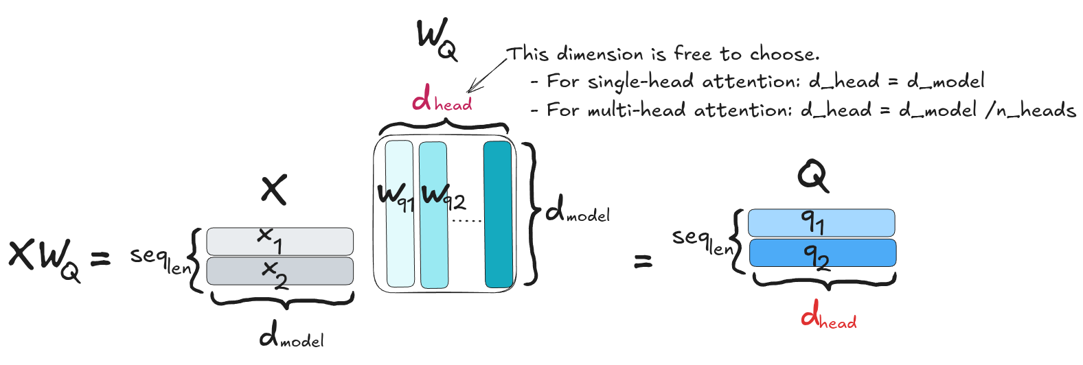
As before, we can use matrix notation to compute all query, key and value vectors in a single pass. By stacking all static input embeddings \(\mathbf{x}_i\) into a sequence matrix \(\mathbf{X}\) we compute \[\mathbf{Q} = \mathbf{X} \cdot \mathbf{W}_Q\] \[\mathbf{K} = \mathbf{X} \cdot \mathbf{W}_K\] \[\mathbf{V} = \mathbf{X} \cdot \mathbf{W}_V\] Each row in the resulting matrices represents the query, key, or value vector for the corresponding input embedding. Figure 9 visualizes the operation \(\mathbf{XW}_Q = \mathbf{Q}\). The matrices \(\mathbf{K}\) and \(\mathbf{V}\) are computed identically using \(\mathbf{W}_K\) and \(\mathbf{W}_V\) . To perform this multiplication, \(\mathbf{W}_Q\) must have \(d_{\text{model}}\) rows, but we are free to choose the number of columns, which we denote as \(d_{\text{head}}\). The resulting query, key, and value vectors will have dimension \(d_{\text{head}}\). In the simplest setup, we set \(d_{\text{head}} = d_{\text{model}}\). This is the single-head attention setup we have been exploring so far. We’ll look at other choices in the follow-up article about multi-head attention.
Abstract Queries vs. Human Questions
Something I personally found confusing when first reading about transformers was the frequent mention of “questions that tokens ask about other tokens.” Without seeing the math behind the analogy, I couldn’t comprehend what these “questions” were or where they came from.
Here, we have already established that these “questions” are query vectors (\(\mathbf{q}_i\))—vectors of numbers, not natural language sentences. They are produced by multiplying a static input embedding \(\mathbf{x}_i\) by \(\mathbf{W}_Q\) (as shown in Section 8). But why is it valid to interpret a query \(\mathbf{q}_i\) as a “question,” other than that it fits nicely into the database analogy?
To see why this claim holds up, let’s look at how a query vector is created. Figure 10 schematically shows a 3-dimensional static embedding \(\mathbf{x}_i\) (colored rectangles) multiplied by \(\mathbf{W}_Q\). The components of \(\mathbf{W}_Q\) are represented as black squares whose sizes correspond to their values: larger squares represent larger weights. To compute \(\mathbf{x}_i \mathbf{W}_Q\), each component of \(\mathbf{x}_i\) is weighted by the corresponding component in \(\mathbf{W}_Q\). The resulting query vector \(\mathbf{q}_i\) (bottom row) consists of the sum of these weighted entries. In other words, the components of \(\mathbf{q}_i\) are the dot products \(\mathbf{x}_i\mathbf{w}_{q,1}\) and \(\mathbf{x}_i \mathbf{w}_{q,2}\). (With \(\mathbf{w}_{q,1}\), and \(\mathbf{w}_{q,2}\) denoting the first and second column vector in \(\mathbf{W}\).)
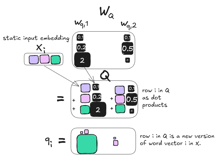
Notice how the first component of \(\mathbf{q}_i\) is dominated by the green entry (the third component of \(\mathbf{x}_i\)), while other components are dampened nearly to zero. We can clearly see how \(\mathbf{W}_Q\) acts as a filter: it can isolate and amplify specific features of \(\mathbf{x}_i\) while silencing others.
So, how does a filtered vector become a “question”?
The answer lies in what happens next when we compute the dot product between a query and a key (\(\mathbf{q}_i \cdot \mathbf{k}_j\)). A dot product outputs a high score only when two vectors share large numbers in the same positions. Because \(\mathbf{W}_Q\) filtered \(\mathbf{x}_i\) to emphasize a specific trait, the resulting vector \(\mathbf{q}_i\) will only match strongly with keys (\(\mathbf{k}_j\)) that possess that exact same trait.
In other words:
- Producing a query vector that isolates a specific feature and then computing the dot product with all keys (as in \(\mathbf{q}_i\mathbf{K}^T\)) is mathematically equivalent to broadcasting: “Who else in this sequence has this feature?”
This is why calling \(\mathbf{q}_i\) a “question” is justified.
How to code single-head attention?
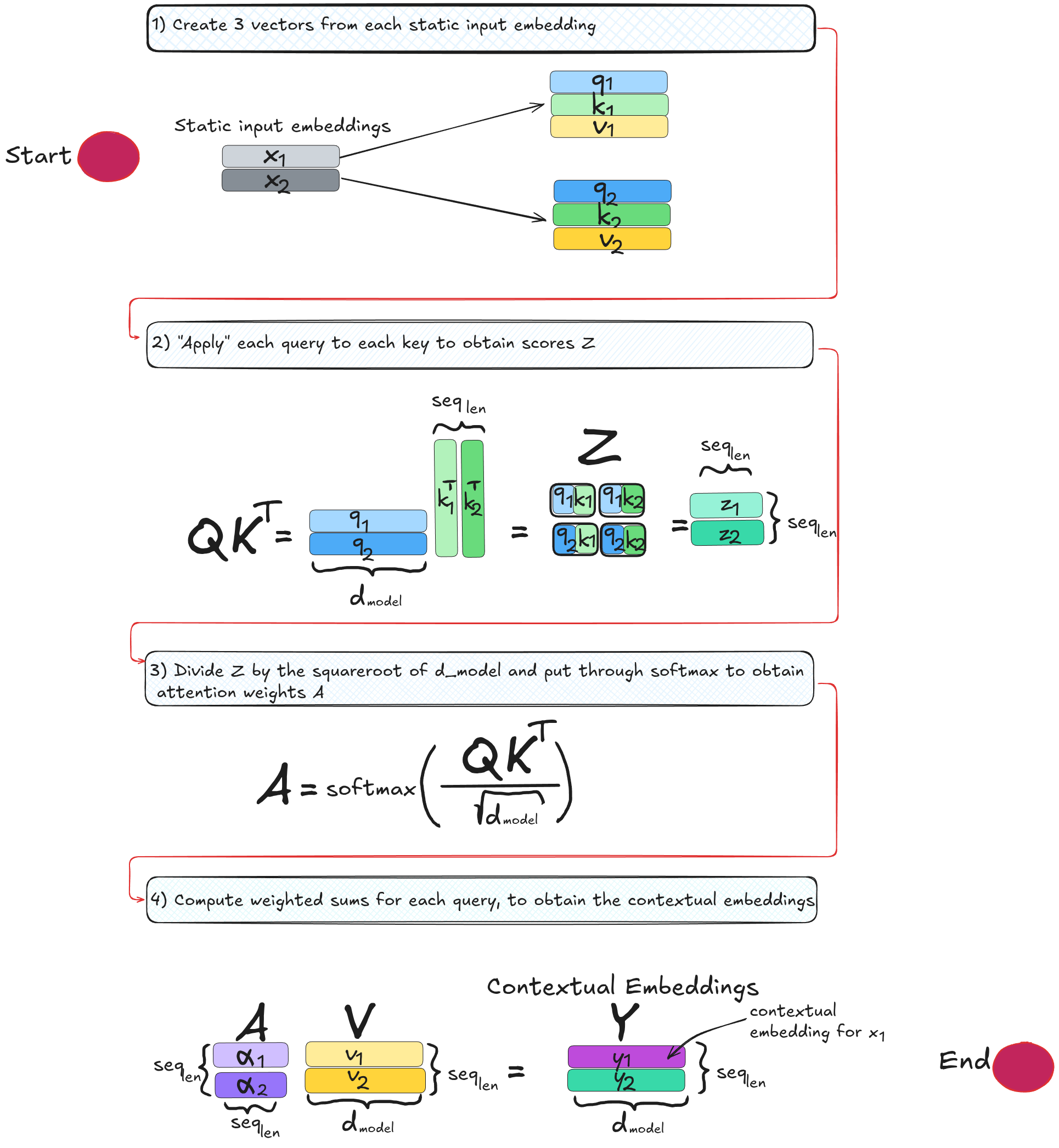
For clarity, here is an overview of the steps involved in scaled dot-product attention:
We can implement this directly in Python using NumPy:
Code
import numpy as np

# Set seed for reproducibility
np.random.seed(42)

# ---------------------------------------------------------------
# Create matrix X with some inputs: 2 words (seq_len=2) with
# embedding dimension d_model=3
# ---------------------------------------------------------------
X_words = np.array([[1.0, 2.0, 3.0],
                    [3.0, 3.0, 2.0]])

seq_len, d_model = X_words.shape

# ---------------------------------------------------------------
# Create the projection matrices whose weights will be learned.
# Matrices shape: (d_model, d_model)
# ---------------------------------------------------------------
W_Q = np.random.randn(d_model, d_model)
W_K = np.random.randn(d_model, d_model)
W_V = np.random.randn(d_model, d_model)

# ---------------------------------------------------------------
# 1) Create 3 vectors from each static input embedding:
# I.e. Linear Projections: Q = X @ W_Q, K = X @ W_K, V = X @ W_V
# Matrix shape:
# (seq_len, d_model) @ (d_model, d_model) -> (seq_len, d_model)
# ---------------------------------------------------------------
Q = X_words @ W_Q
K = X_words @ W_K
V = X_words @ W_V

print("Queries (Q):\n", Q, "\n")
print("Keys (K):\n", K, "\n")
print("Values (V):\n", V, "\n")

# ---------------------------------------------------------------
# 2) Apply each query to each key to obtain scores
# I.e.  Unscaled Dot-Products & Variance Scaling
# Matrix shape:
# (seq_len, d_model) @ (d_model, seq_len) -> (seq_len, seq_len)
# ---------------------------------------------------------------
scores_raw = Q @ K.T

# ---------------------------------------------------------------
# 3) Scale and Normalize
# Convert raw similarity scores into row-wise probability
# distribution
# ---------------------------------------------------------------
scores_scaled = scores_raw / np.sqrt(d_model)
def softmax(x):
    exp_x = np.exp(x - np.max(x, axis=-1, keepdims=True))  # Numerical stability trick
    return exp_x / exp_x.sum(axis=-1, keepdims=True)

A = softmax(scores_scaled)
print("Attention Weights Matrix (A):\n", A, "\n")

# ---------------------------------------------------------------
# 4) Compute weighted sum
# I.e. Final Output Matrix (Y = A @ V)
# Matrix shape:
# (seq_len, seq_len) @ (seq_len, d_model) -> (seq_len, d_model)
# ---------------------------------------------------------------
Y = A @ V
print("Contextualized Output Embeddings (Y):\n", Y)
Queries (Q):
[[ 8.28041231 1.69573314 -1.22900853]
[ 9.21765766 0.41761643 0.30170597]]
Keys (K):
[[-0.660378 -7.32847154 -2.97282342]
[ 1.22899189 -9.15575605 -5.94344809]]
Values (V):
[[-2.99272485 -0.94447952 -4.83682834]
[-4.49016658 -3.81248131 -2.17928541]]
Attention Weights Matrix (A):
[[8.68363148e-05 9.99913164e-01]
[1.12005616e-04 9.99887994e-01]]
Contextualized Output Embeddings (Y):
[[-4.49003654 -3.81223226 -2.17951618]
[-4.48999886 -3.81216008 -2.17958307]]In practice, you won’t need to write the attention steps manually. Frameworks like PyTorch provide optimized implementations of the mechanism. Note that PyTorch expects inputs to include a batch dimension. Here, we wrap our single input sequence in a batch of size 1:
Code
import torch
import torch.nn as nn

# Set seed for reproducibility
torch.manual_seed(42)

# ---------------------------------------------------------------
# Create matrix X with some inputs: 2 words (seq_len=2) with
# embedding dimension d_model=3
# ---------------------------------------------------------------
X_words = torch.tensor([[1.0, 2.0, 3.0],
                    [3.0, 3.0, 2.0]])

seq_len, d_model = X_words.shape


# ---------------------------------------------------------------
# PyTorch layers expect batched inputs:
# (batch_size, sequence_length, d_model)
# ---------------------------------------------------------------
X_batch = X_words.unsqueeze(0)  # Shape becomes [1, 2, 3]

# ---------------------------------------------------------------
# Instantiate PyTorch's MultiheadAttention with num_heads=1 for
# single-head batch_first=True expects
# shape: (batch_size, sequence_length, d_model)
# ---------------------------------------------------------------
attn_layer = nn.MultiheadAttention(embed_dim=d_model, num_heads=1, batch_first=True)

# ---------------------------------------------------------------
# Compute Self-Attention (passing X in for Query, Key, and Value)
# Now torch does all the required work and simply
# spits out the contextualized embeddings as Y.
# Returns: (contextualized_outputs, attention_weights)
# ---------------------------------------------------------------
Y_batch, A_batch = attn_layer(query=X_batch, key=X_batch, value=X_batch)

# ---------------------------------------------------------------
# Remove the batch dimension for inspection
# ---------------------------------------------------------------
Y = Y_batch.squeeze(0)
A = A_batch.squeeze(0)

print("Attention Weights Matrix (A):\n", A.detach().numpy(), "\n")
print("Contextualized Output Embeddings (Y):\n", Y.detach().numpy())
Attention Weights Matrix (A):
[[0.8597921 0.14020787]
[0.91717255 0.08282746]]
Contextualized Output Embeddings (Y):
[[0.703761 0.64951515 0.80751586]
[0.7178543 0.6376342 0.79714787]]Important Note on Numerical Outputs: If you compare the output matrix \(Y\) from the NumPy implementation to the PyTorch results, you will notice the numbers differ, for two reasons. First, even though we set np.random.seed(42) and torch.manual_seed(42), NumPy and PyTorch use different underlying algorithms for pseudo-random number generation, so the initialized projection weights (\(W_Q, W_K, W_V\)) start from different raw values. Second, the nn.MultiheadAttention module doesn’t stop at \(\mathbf{AV}\): it passes the result through one more learned linear layer (out_proj) before returning it. This extra projection is a real part of the transformer architecture—we simply haven’t introduced it yet, since it only becomes relevant once we combine multiple attention passes, which is exactly the subject of the follow-up article. For now, just be aware that the PyTorch output isn’t our formula with different weights; it’s our formula plus one additional learned step on top.
Summary
As promised in the introduction, we have tackled both the how and the why of single-head scaled dot-product attention. We have seen how attention transforms static input embeddings into contextualized representations (summarized in Figure 11).
We now also understand why each step takes place:
- Query, key, and value vectors are created via learned linear projections (\(\mathbf{W}_Q, \mathbf{W}_K, \mathbf{W}_V\)). Their purpose is to construct weighted averages of the input vectors. Their names come from the database analogy.
- Queries act as feature filters—asking “questions” about other tokens—which is realized mathematically through the score matrix \(\mathbf{QK}^T\).
- Scaling by \(\sqrt{d_{\text{model}}}\) prevents numerical instability and softmax saturation by keeping score variance constant regardless of embedding size.
- Softmax converts these scaled scores into row-wise probability distributions (attention weights) between 0 and 1 that sum to 1.
- Multiplying by \(\mathbf{V}\) forms the weighted sum of the value vectors attached to each token.
Thus, for Single-Head Scaled Dot-Product Attention, we have:
\[\text{Attention}(\mathbf{Q}, \mathbf{K}, \mathbf{V}) = \text{softmax}\left(\frac{\mathbf{QK}^T}{\sqrt{d_{\text{model}}}}\right)\mathbf{V}\]
What’s Next?
While a single attention pass is powerful, it has a major shortcoming: it produces only one query vector per static input embedding. Thus, each token can ask exactly one question.
In natural language, a single question is rarely enough to capture every contextual nuance. A token might need to ask one question about grammatical structure and another about semantic meaning. In the next article, we will see how running multiple attention passes in parallel—a setup known as Multi-Head Attention—solves this by allowing the model to project inputs into several feature spaces at once.
References
Discover more from Master the Math
Subscribe to get the latest posts sent to your email.