

Linear regression is often used as the “Hello World” of deep learning—the very first example to introduce concepts of artificial neural networks, and thus a fundamental concept in machine learning (ML). However, the method is deeply rooted in statistics, dating back to the early 18th century. Since the same problem is tackled from two different perspectives (statistics and ML), different terms exist for similar concepts, and different aspects are emphasized depending on whether you’re team statistics or team machine learning.
Inevitably, this can get confusing, so it’s worthwhile to take a closer look at the overlap and distinctions between both approaches. In this article, we’ll understand the basics of linear regression from a statistical perspective (where I put the focus) and contrast them with the machine learning view. We’ll cover what
regression analysis is about,
simple linear regression is,
the normal error regression model is,
and how it’s vectorized for efficient computation.
I’ll briefly sketch the methods used to compute the model parameters.
The post is beginner-friendly but requires some basic statistical knowledge, such as random variables, parameter estimation (covered here), and confidence intervals (introduced here). You’ll also need basic linear algebra knowledge to follow the vectorization parts. The main resources for this article were [1], [2], and [3].
What is regression analysis?
Regression analysis is about:
Predicting a numerical (continuous) variable using one (simple regression) or several other numerical variables (multiple regression).
Investigating whether there’s a relationship between one or several numerical variables and, if so, what it looks like.
Making statements about how trustworthy possible predictions are.
For example, can you estimate a person’s weight if you know their height? You probably reason that, on average, taller people are heavier than shorter ones. But how much heavier? And is this assumption even correct? To investigate systematically, we need to formalize the problem.
First, we model “height” (\(X\)) and “weight” (\(Y\)) as quantitative random variables taking numerical values (as opposed to categorical variables that take values like “red”, “green”, “hot”, “cold”, etc.). Next, we observe a specific height value \(x\) (the specific value that a random variable can take is usually denoted as a lowercase letter; for example, \(X = x\) indicates that the random variable \(X\) takes the value \(x\)) and wonder if we can make a statement about the person’s weight given that height.
This can be formalized as a conditional probability problem: what is the conditional distribution of weight given a particular height observation? That is, \[P(Y = y \mid X = x).\] This is the focus of regression analysis: it provides the framework to study whether there’s a relationship between one quantitative variable and another (or multiple others), and what that relationship looks like.
Linear regression in machine learning vs. statistics
In ML, linear regression is considered a simple problem that’s just complicated enough to introduce the basics of the ML pipeline for artificial neural networks. Thus, it illustrates the well-known procedure: choose a model and a loss function to create an optimization problem that you solve with an appropriate strategy—usually gradient descent. Then the backpropagation algorithm that efficiently computes the gradients (for gradient descent) is introduced, along with how to avoid artifacts like over- or underfitting and how to evaluate model performance. As already stated, the focus is on introducing the ML pipeline. The “learning” is considered done once the model makes good enough predictions on test data.
In statistics, we approach the problem from the field of Statistical Inference. We interpret the data as a sample (a small observation) of the population (the entire data, which is unfortunately unavailable). We assume the population was produced by a model or process with parameters that we can’t know exactly but can only estimate from the available sample. Parameter estimation is what Statistical Inference is about. Therefore, we aim for parameter estimation rather than learning weights.
In particular, as statisticians, we don’t settle for “good enough” predictions. We seek optimal estimates and—importantly—quantify how good they are using techniques like confidence intervals and hypothesis tests. To accomplish this, statisticians emphasize the noise, i.e., the inability to perfectly predict the dependent variable from the independent one. ML often ignores this or treats it only implicitly.
Also, the mean squared error (the difference between prediction and actual observed value) is not just an intuitive loss (as it’s often treated in ML). In statistics, it’s derived as the expected value of the squared difference between prediction and truth, connecting to the bias–variance decomposition [4].
Summing up, statisticians’ methods are theoretically well justified. In ML literature, the same concepts may be used, but often—not always—the reader is spared the heavy theory.
The terms and notations in ML also differ slightly from those in statistics. I’ll point out differences throughout the text.
What is simple linear regression?
Consider a simple numerical example to illustrate. Suppose you’ve measured the heights and weights of 10 people (in cm and kg), as shown in Table 1.
| person | height (\(X\)) | weight (\(Y\)) |
|---|---|---|
| 1 | 186 | 90 |
| 2 | 174 | 70 |
| 3 | 186 | 93 |
| 4 | 176 | 82 |
| 5 | 182 | 89 |
| 6 | 176 | 80 |
| 7 | 184 | 86 |
| 8 | 176 | 79 |
| 9 | 179 | 85 |
| 10 | 186 | 98 |
We call the variable to be predicted the dependent variable or response \(Y\), and the variable used for prediction the predictor, independent, or explanatory variable \(X\). In ML, these are typically called “input” and “output” variables. In our example, height is the predictor and weight the response. A problem involving only one predictor is called simple linear regression. When more than one predictor is involved, we speak of multiple linear regression.
Regression analysis doesn’t magically reveal the true relationship; instead, we assume a form for that relationship and evaluate how well it fits the data. In linear regression, we assume this relationship is linear. Thus, simple linear regression (SLR) assumes one numerical variable can be predicted from another via a linear relationship.
The data in Table 1 is a sample from a larger population. Sample and population are fundamental concepts in statistics; the sample is used to make inferences about population parameters. In ML, the same sample is called “training data.” The columns are variables (or “features” in ML). Each row is one observation. In statistics, the \(i\)th observation is denoted by a subscript; in ML, often a superscript in round parentheses is used, e.g., \(x^{(i)}\). The round parentheses distinguish it from an exponent. In the following, I’ll borrow the ML notation (superscript) because I find it more convenient.
Regression analysis is concerned with statistical relations
We distinguish between two types of relations between two variables:
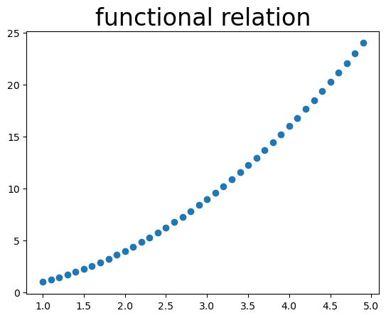
A functional relation (or deterministic relation) is of the form \(Y = f(X)\), where the same \(x\) always maps to the same \(y\). For example, in \(y = 3x\), when \(x = 2\), \(y\) is always 6.
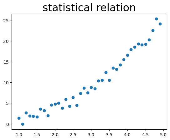
A statistical relation, in contrast, is one where the same \(X\) value can correspond to different \(Y\) values due to random variation. For example, \(x = 2\) might yield \(y = 6\) in one observation and \(y = 6.5\) in another, even though the central tendency lies along a line.
This is illustrated in Figure 1, which shows a functional relation (top) and a statistical relation (bottom). In the statistical case, the \(y\)-values are not completely random; they roughly follow a line but scatter around it. Such a plot is called a scatterplot. Regression analysis concerns statistical relations of this kind and aims to find the line (or more general function) that the observed values scatter around. This line is the regression function. In simple linear regression, it’s a straight line.
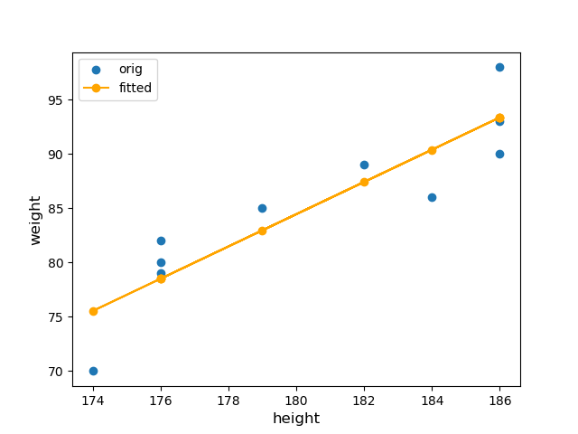
In Figure 2, we apply this to our example. The blue points correspond to the data in Table 1. They form a statistical relation: the same \(x\)-values appear with different \(y\)-values, and the points scatter around a line (shown in orange). This orange line is the regression line for simple linear regression.
The simple (linear) regression model and the normal error regression model
As just stated, in simple linear regression, the regression function is a line (other regression models assume different functional forms). A line can be described by the equation \[Y = mX + b,\] where \(m\) is the slope and \(b\) the \(y\)-intercept. In regression, \(X\) is the independent (predictor) variable and \(Y\) the dependent (response) variable. We treat \(Y\) as a random variable that takes specific values. In contrast, in the standard simple linear regression model, the predictor \(X\) is treated as fixed (non-random).
It is also possible—and sometimes necessary—to treat \(X\) itself as random; in this case, the model is often called a correlation model, in contrast to the standard regression model where \(X\) is fixed and only \(Y\) is random [1].
In our example, the pairs \((x^{(i)}, y^{(i)})\) are the height–weight measurements. Each \(x^{(i)}\) is the value of the \(i\)th observation of the predictor, e.g., \(x^{(1)} = 186\) and \(y^{(1)} = 90\). The line equation captures the deterministic part of the relationship but doesn’t account for the scatter around the line observed in the data.
To incorporate this scatter, we add a random error term \(\epsilon\): \[\begin{equation} y^{(i)} = \beta_0 + \beta_1 x^{(i)} + \epsilon^{(i)}. \label{eq:normmod} \end{equation}\]
Here, \(\beta_1\) is the slope and \(\beta_0\) the \(y\)-intercept. Denoting these parameters \(\beta\) is common in statistics; they are the regression coefficients. In ML, we’d call them “weights” and denote them \(\omega_0\) and \(\omega_1\). The term \(\epsilon^{(i)}\) represents the noise or error, modeled as a random variable. The main task in regression analysis is to estimate these coefficients from the data.
Note that adding the noise is a design choice; we could incorporate it differently, e.g., by multiplying the \(y\)-value by \(\epsilon\) (“multiplicative noise”). However, in SLR, the simple assumption is additive noise.
We make these assumptions about the errors and their distribution:
All \(\epsilon^{(i)}\) follow the same distribution.
This distribution has mean zero: \(E[\epsilon^{(i)}] = 0\).
This distribution has constant but unknown variance \(\sigma^2\).
The errors are uncorrelated: no linear relationship between \(\epsilon^{(i)}\) and \(\epsilon^{(j)}\) for \(i \neq j\) (covariance is 0; this doesn’t imply independence).
The property that error terms have the same (unknown) variance is called homoscedasticity. Models satisfying these assumptions are simple linear regression models. If we additionally assume the \(\epsilon^{(i)}\) are independent and normally distributed, \[\epsilon^{(i)} \sim \mathcal{N}(0, \sigma^2),\] the model in (1) becomes the normal error regression model, a more specific version.
A useful mnemonic for the assumptions of the normal error regression model is the word LINE [2]:
L—the model is linear in the parameters \(\beta_0, \beta_1\).
I—the errors are independent of each other.
N—the errors follow a normal distribution with zero mean.
E—the errors have equal variances (homoscedasticity).
(Test yourself: What’s the difference between the normal regression model and the regression function? What assumptions are made about the error in the normal error regression model? What is homoscedasticity?)
Vectorization
Vectorization means rewriting the model using linear algebra so sums become matrix–vector operations. This is important both mathematically and computationally:
It allows more concise, clean equations.
Matrix operations are highly parallelizable and can be accelerated on GPUs.
In programming, vectorization often means rewriting loops as array operations in libraries like NumPy, which is simpler and faster.
We use these notations:
Matrices: bold uppercase, e.g., \(\mathbf{A}\).
Vectors: bold lowercase, e.g., \(\mathbf{x}\); all column vectors.
Scalars: regular lowercase, e.g., \(a\).
So far, our model (1) was for a single observation. For \(n\) observations, we write the responses as a vector: \[\begin{equation} \mathbf{y} = \beta_0 + \beta_1 \mathbf{x} + \boldsymbol{\epsilon} = \begin{bmatrix} y^{(1)} \\ \vdots \\ y^{(n)} \end{bmatrix} = \beta_0 + \beta_1 \begin{bmatrix} x^{(1)} \\ \vdots \\ x^{(n)} \end{bmatrix} + \begin{bmatrix} \epsilon^{(1)} \\ \vdots \\ \epsilon^{(n)} \end{bmatrix}. \label{eq:vec_eq} \end{equation}\]
This can be written more concisely by incorporating the intercept into a matrix form. We define the design matrix as \[\mathbf{X} = \begin{bmatrix} 1 & x^{(1)} \\ \vdots & \vdots \\ 1 & x^{(n)} \end{bmatrix},\] and the parameter vector as \[\boldsymbol{\beta} = \begin{bmatrix} \beta_0 \\ \beta_1 \end{bmatrix}.\] Then the model becomes \[\begin{equation} \mathbf{y} = \mathbf{X}\boldsymbol{\beta} + \boldsymbol{\epsilon}. \label{eq:matrix_model} \end{equation}\]
Here, the unknowns are the regression coefficients \(\beta_0, \beta_1\) and error variance \(\sigma^2\), which we’ll estimate from the data.
(Test yourself: Why do we need vectorization? What is the design matrix?)
Vectorization for MLR
In ML literature, you’ll often see \[y = \mathbf{w}^\top \mathbf{x} + \varepsilon, \quad \varepsilon \sim \mathcal{N}(0, \sigma^2).\] This differs slightly from our vectorized expression because it concerns multiple linear regression: each scalar \(y^{(i)}\) is computed not from a scalar \(x^{(i)}\) (as in simple linear regression) but from a vector \(\mathbf{x}^{(i)}\). In ML terms, we use various features to predict \(y^{(i)}\). For example, predict weight from height and age: \(\mathbf{x}^{(i)} = [x_1, x_2]^\top\), where \(x_1 =\) height and \(x_2 =\) age.
For two features: \[y^{(i)} = \beta_0 \cdot 1 + \beta_1 x_1^{(i)} + \beta_2 x_2^{(i)} + \varepsilon^{(i)}.\] Replacing \(\beta_i\) with \(w_i\) and writing as a vector: \(y^{(i)} = \mathbf{w}^\top \mathbf{x}^{(i)} + \epsilon^{(i)}\), where \[\mathbf{w} = \begin{bmatrix} w_0 \\ w_1 \\ w_2 \end{bmatrix}, \quad \mathbf{x}^{(i)} = \begin{bmatrix} 1 \\ x_1 \\ x_2 \end{bmatrix}.\]
This is for a single observation (superscript \(i\)). For the entire dataset: \[\mathbf{y} = \mathbf{X}\mathbf{w} + \boldsymbol{\epsilon},\] where each row of \(\mathbf{X}\) is an observation of the \(x\) values for a single \(y\). For our two-feature example: \[\mathbf{X} = \begin{bmatrix} 1 & x_1^{(1)} & x_2^{(1)} \\ 1 & x_1^{(2)} & x_2^{(2)} \\ \vdots & \vdots & \vdots \\ 1 & x_1^{(N)} & x_2^{(N)} \end{bmatrix}.\]
Alternative regression model
For completeness, there’s an alternative form of the simple linear regression model where we subtract the mean of \(x^{(i)}\). Here, the \(y\)-intercept represents the predicted value at the mean of \(x\) rather than at \(x=0\): \[y^{(i)} = \beta_0^{*} + \beta_1 (x^{(i)} – \bar{x}) + \epsilon^{(i)},\] with \(\beta_0^{*} = \beta_0 + \beta_1 \bar{x}\). Here, \(\beta_0^{*}\) is the predicted value at \(\bar{x}\), and \(\beta_1\) is unchanged. Both forms are equivalent; choose based on interpretability (intercept at \(x=0\) or data center).
Implications of the normal error regression model
We’ve defined the normal error regression model as \[\mathbf{y} = \mathbf{X}\boldsymbol{\beta} + \boldsymbol{\epsilon}, \quad \boldsymbol{\epsilon} \sim \mathcal{N}(\mathbf{0}, \sigma^2 \mathbf{I}),\] where errors are independent, identically distributed normals with zero mean and constant variance \(\sigma^2\). Since functions of random variables are random variables, and \(y^{(i)}\) are linear functions of \(\epsilon^{(i)}\), each \(y^{(i)}\) is normally distributed: \[E[y^{(i)}] = \beta_0 + \beta_1 x^{(i)}, \quad \mathop{\mathrm{Var}}(y^{(i)}) = \sigma^2.\] The regression function—the line \(y = \beta_0 + \beta_1 x\)—is thus the expected value of the response at each predictor level. Dropping the error from equation 3 gives this “central line” around which data points scatter.
Figure 3 (adapted from [1]) visualizes this. Each \(y^{(i)}\) lies in a band around \(E[y^{(i)}]\), with distance determined by \(\epsilon^{(i)}\). The arcs depict underlying normal densities centered at predicted means.
![Figure 3: Visualization of the normal error linear regression model. Here, \alpha corresponds to \beta_0 and \beta to \beta_1. Each y^{(i)} lies within a band around E[y^{(i)}], determined by \epsilon^{(i)}.](https://markelic.de/wp-content/uploads/2026/04/visual_regression_model.png)
(Test yourself: What’s the difference between the normal regression model and regression function? What error assumptions in the normal error model? What is the regression function?)
Be careful when you look at values beyond the scope of the model
Recall our example in Figure 2. The data has \(x \geq 0\); the model was fit only there. Extending the fitted line to negative \(x\) may not make sense—predicting weight from negative height gives a meaningless negative number. This shows we must be cautious interpreting beyond the model’s scope (range of \(x\)-values used to fit it).
Outlook: estimating regression coefficients vs. learning weights
Now we turn to regression analysis’s core task: estimating unknown parameters \(\beta_0\) and \(\beta_1\) from data. Since this article is already long, I’ll only sketch an outlook.
In statistics, these are parameters of an underlying data-generating process; in ML, they’re often weights or learned parameters.
Let’s look at the statistical perspective first: With only a population sample, we can’t know true values exactly, so we compute point estimates via criterion functions (criterion functions are the term that statisticians use for cost, loss, or objective functions, where the three latter names are often used by the ML community). Two common approaches are:
Least Squares: Uses model form without distributional assumptions. Minimizes sum of squared residuals: \[S(\beta_0, \beta_1) = \sum_{i=1}^n \bigl( y^{(i)} – \beta_0 – \beta_1 x^{(i)} \bigr)^2.\] Result: ordinary least squares (OLS) estimators.
Maximum Likelihood Estimation (MLE): Uses normal error model. Maximizes data likelihood under normal errors. For normal errors, MLE of \(\beta_0, \beta_1\) coincides with OLS; \(\sigma^2\) MLE relates to residual variance.
In statistics, estimation doesn’t stop at point estimates. We construct confidence intervals for coefficients (and predictions) to quantify uncertainty, derived from estimated error variance and normal error assumptions. Alternatively, we test hypotheses about estimated values.
In machine learning, the same goal—finding good values for the coefficients—can be approached differently. Instead of solving the least squares problem in closed form or via maximum likelihood, one can frame the task as an optimization problem and use a neural network or a simple linear model with iterative optimization (e.g., gradient descent). The model is then trained on the data until the predictions are sufficiently accurate.
Summary
Congratulations on making it this far. We’ve covered simple linear regression basics and contrasted statistical and machine learning approaches.
Simple linear regression assumes a linear relationship between two numerical variables and predicts one (dependent) from the other (independent).
Statistics makes assumptions about the model (emphasizing error via “normal error model”: additive normal noise). It stresses uncertainty (LINE: Linear, Independent, Normal, Equal variance) and goes beyond estimating coefficients (slope, \(y\)-intercept) to confidence intervals.
In ML, it’s an entry point for deep learning: coefficients are weights learned via optimization (backpropagation, gradient descent), typically settling for point estimates without confidence intervals.
Distinguishing these perspectives helps you orient yourself. Knowing an author’s viewpoint tells you what to expect and where to find further reading on statistics-heavy or ML-focused topics.