
The method of maximum likelihood estimation allows to estimate point parameters for a given distribution underlying some observed data. Let’s look at an example to understand what this means:
Imagine you measure the height of 20 women within an age-range between 20-40 years. You denote the measurements as $X_1=x_1, X_2=x_2,…,X_{20}=x_{20}$, where the capital $X_i$ refers to the i’th measurement and the lowercase $x_i$ to the particular value. For example, if the third measurement was 164 centimeters, you write $X_3=164$, so $x_3=164$. Each measurement can be interpreted as an outcome of a random experiment. Therefore, we can interpret each $X_i$ as a random variable, r.v., and each $x_i$ as a sample drawn from the (one) distribution that we associate with the random variables. Again – we believe that all $X_i$ follow the same probability distribution. In other words, we have a random sample from an unknown joint probability distribution. Notice also that the height of one woman is independent of the height of another woman. Therefore, we can also assume that the measurements are mutually independent of each other. We call a set of r.v.s with these properties (mutual independence and sharing the same distribution), independent and identically distributed, i.i.d..
In this example, we assume that the joint probability distribution of our random sample is a normal distribution. This assumption is our model hypothesis. A normal distribution is determined by its mean $\mu$ and variance $\sigma^2$. Unfortunately, we do not know these parameters. Of course, we could assume another distribution if we had a good reason to do so, and in that case we would have a different set of unknown parameters to estimate. Now we want to find good estimates for those unknown parameters. This is what Maximum Likelihood Estimation does: It finds the (point) estimates of the model parameters that make the observations most likely (→ maximally likely → maximum likelihood). Most likely means: It chooses the parameters for which the joint probability for the observations
is maximal. So the word ”likelihood” is not the same as ”probability”. A probability can be determined/described by a pmf/pdf. For example, $P(X = x)$, the probability that the r.v. X takes the value x is defined by its according pmf=$f_X(x)$ (or pdf in the continuous case), which could be a function governed by one (or more) parameter(s), θ. The task is to find a value for θ s.t. P (X = x) is maximal. Let’s check figure 1 to see an example for that:
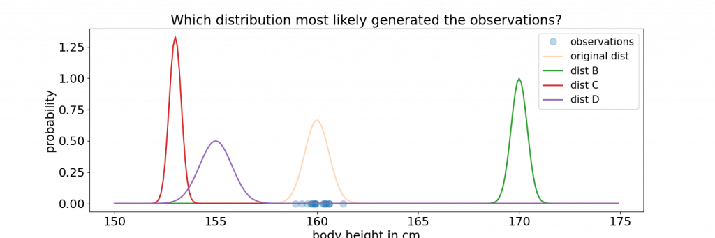
distribution is most likely to have produced these observations?
The blue crosses denote the 20 height measurements from our example. These observations were drawn from the normal distribution plotted in pale orange. In reality we would not know this distribution and/or its parameters. Suppose, we had been given 3 other normal distributions, B, C, and D, plotted in green, red, and purple in the figure. Which one of these 3 distributions is most likely to have produced the observations? By eyeballing it, we can tell it is the one plotted in purple (although none of these three given distributions really looks appropriate). How to quantify this? We want to know the probability of obtaining the given observations under the assumption that they were generated by each of the 3 given distributions. So we are asking: ”What is the probability that the event $X_1 = x_1$ and the event $X_2 = x-2 $and … $X_{20} = x_{20}$ occur together, given that they were all generated by distribution B”. This can be written as: $P(X_1=x_1 \cap … X_{20}=x_{20} | \mu_{B}; \sigma_{B})$. In this case, the subscript B denotes the parameters of the particular distribution. We simply compute this probability for all the three distributions, and then we pick the distribution for which we got the highest probability. Remember: the $X_i$ are i.i.d.. The joint probabilty of n events is the product of the probability of each individual event, if the events are independent. Because i.i.d. implies independence we can write our probability as a product as shown in equation 1.
\begin{equation}
  \begin{aligned}
    &P(X_1=x_1 \cap ... X_{20}=x_{20} | \mu_{B}; \sigma_{B}) \\
    &= P(X_1=x_1| \mu_{B}; \sigma_{B}) P(X_2=x_2  | \mu_{B}; \sigma_{B}) ... P(X_{20}=x_{20} | \mu_{B}; \sigma_{B}) \\
    &= f_X(x_1| \mu_{B}; \sigma_{B}) f_X(x_2  | \mu_{B}; \sigma_{B}) ... f_X(x_{20} | \mu_{B}; \sigma_{B}) \\
    &= \prod_{i=1}^{20} f_X(x_i | \mu_{B}; \sigma_{B})
  \end{aligned}
  \end{equation}
To compute the probability of $P(X_1 = x_1 |\mu_B ; \sigma_B ) $we need to plug in $\mu_{B}$ and $\sigma_{B}$ into the formula for the normal distribution:
  \begin{equation}
  \begin{aligned}
P(X_1=x_1 | \mu_{B}; \sigma_{B} )= \frac{1}{\sqrt{2\pi} \sigma_B}  e^{(\frac{-1}{2})  (\frac{x_1 - \mu_B}{\sigma_B})^2}
  \end{aligned}
  \end{equation}
The probabilites $P(\textbf{X} | \mu_{j}; \sigma_{j} )$ – where X denotes a vector of all measurements and the subscript $j$ takes the values “B”, “C”, and “D”, to make the expression more compact – can easily be computed with software. The following shows the code for Python.
import scipy.stats as stats
import numpy as np

# Generate a normal distribution with given mu=160 and sigma=0.6.
norm_a = stats.norm(loc=160, scale=0.6)

# Draw many samples of that distribution. These are the observations x_i.
observations = norm_a.rvs(20,random_state=12)

# Generate 3 more normal distributions with different values for mu and
# sigma.
norm_b = stats.norm(loc=170, scale=0.4)
norm_c = stats.norm(loc=153, scale=0.3)
norm_d = stats.norm(loc=155, scale=0.8)

# Compute the probabilities that the observations were generated by each
# distribution.
p_dist_B = np.prod(norm_b.pdf(observations))
p_dist_C = np.prod(norm_c.pdf(observations))
p_dist_D = np.prod(norm_d.pdf(observations))
print(f"Likelihood that observations produced by dist_B: {p_dist_B}")
print(f"Likelihood that observations produced by dist_C: {p_dist_C}")
print(f"Likelihood that observations produced by dist_D: {p_dist_D}")

#Likelihood that observations produced by dist_B: 0.0
#Likelihood that observations produced by dist_C: 0.0
#Likelihood that observations produced by
#dist_D: 5.31599875483204e-181
We notice that the results are 0 or very close to 0. This is because we are multiplying many very small numbers. But we see that the highest likelihood is computed for distribution D, which corresponds to the purple plot in the figure above. So, now we don’t have to eyeball anymore, but have a way to quantify this result numerically.
Thus far, we have seen an example which helped us to understand what is meant by: “estimating the parameters that make our observations most likely”. Of course, the above is not very helpful, because none of the three distributions explain our random sample well. Its purpose was to merely give us an intuition of what needs to be computed.
We have seen that the input to MLE is a set of values (the observations) interpreted as a random sample of i.i.d. r.v.s, and a model we assume reasonable. The output will be an optimal set of parameters, in the sense that it maximizes the likelihood of our observations under the assumption of the given model. A sketch of in- and output of MLE is shown in fig. 2
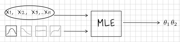
parameters.
In the above example, we only computed three different likelihoods for three different parameter sets for a normal distribution. To improve our estimate, we could assume many more parameter sets and compute the likelihoods for each of them. However, this is computationally expensive. It’s more efficient to use calculus. Calculus tells us how to find the parameters of a function for which the function value is maximal or minimal. If you don’t remember this, you might want to review calculus I material. We find extreme values of a function (min, max, or saddle point), where the slope is 0. The slope of a function is given by its first derivative. So we need to derive the function, set it to 0, and compute the parameter values for that. To see if we found a maximum for such a paramter set, we need to compute the second derivative at that position; if the result is a negative number, we found a (relative) maximum.
The likelihood function
The first thing we need in order to use calculus is a function that we want to optimize. For our example, this function is given by equation 3 and is called the likelihood function, $\mathcal{L}$.
\begin{equation}
  \begin{aligned}
    \mathcal{L}(\mu,\sigma)&= \prod_{i=1}^{n} f_X(x_i | \mu; \sigma)
  \end{aligned}

\end{equation}
What we want to compute is:
\begin{equation}
  \begin{aligned}
  \underset{\sigma,\mu}{\arg\max} \mathcal{L}(\mu,\sigma),
  \end{aligned}
\end{equation}
Next, we come to an important point: The result of this equation 3 does not change if you take its logarithm, because the logarithm is a monotonically increasing function. In addition, because $log(ab) = log(a)+log(b)$, the product in the equation turns into a sum. This is convenient, but more important is that with this you eliminate the potential underflow that might occur due the multiplication of very small numbers. The logarithm of our likelihood function is given in eq. 5.
\begin{equation}
\begin{aligned}
  &L\left( \mu ,\sigma \right) =\log \left( \prod ^{n}_{i=1}\dfrac{1}{\sqrt{2\pi }\sigma }\exp \left( \dfrac{-\left( x_{i}-\mu \right) ^{2}}{2\sigma ^{2}}\right) \right)= \\
  &\log \left( \left( 2\pi \right) ^{-1/2}\right) +\log \left( \sigma ^{-1}\right) +\log \left( \exp \left( \dfrac{-1}{2}\left( \dfrac{x_{1}-\mu }{\sigma }\right) ^{2}\right) \right)+ \\
  &\log \left( \left( 2\pi \right) ^{-1/2}\right) +\log \left( \sigma ^{-1}\right) +\log \left( \exp \left( \dfrac{-1}{2}\left( \dfrac{x_{2}-\mu }{\sigma }\right) ^{2}\right) \right)+\ldots \\
  &\log \left( \left( 2\pi \right) ^{-1/2}\right) +\log \left( \sigma ^{-1}\right) +\log \left( \exp \left( \dfrac{-1}{2}\left( \dfrac{x_{n}-\mu }{\sigma }\right) ^{2}\right) \right)  = \\
  &n\left( -\dfrac{1}{2}\right) \log \left( 2\pi \right) -n\log \left( \sigma \right) -\dfrac{1}{2}\left( \dfrac{x_{1}-\mu }{\sigma }\right) ^{2}-\dfrac{1}{2}\left( \dfrac{x_{2}-\mu }{\sigma }\right) ^{2}-\ldots -\dfrac{1}{2}\left( \dfrac{x_{n}-\mu }{\sigma }\right) ^{2}=\\
  &n\left( -\dfrac{1}{2}\right) \log \left( 2\pi \right) -n\log \left( \sigma \right)  -\dfrac{1}{2\sigma ^{2}}\sum ^{n}_{i=1}\left( x_{i}-\mu \right) ^{2}
\end{aligned}
\end{equation}
The next step is to take the derivative of the logarithm of the likelihood function. We start with taking the derivative w.r.t. $\mu$:
\begin{equation}
\begin{aligned}
  &\frac{\partial}{\partial \mu}\left( n\left( -\dfrac{1}{2}\right) \log \left( 2\pi \right) -n\log \left( \sigma \right)  -\dfrac{1}{2\sigma ^{2}}\sum ^{n}_{i=1}\left( x_{i}-\mu \right) ^{2}\right)=\\
  &\dfrac{1}{\sigma ^{2}}\left( \sum ^{n}_{i=1}\left( x_{i}-\mu \right) \right)
\end{aligned}
\end{equation}
Finally, set the derivative to 0 and solve for $\mu$. The resulting expression is the value for $\mu$ that maximizes the likelihood function. The expression is called the maximum likelihood estimator for $\mu$, and we distinguish the estimator from the true value by marking it with the hat symbol, i.e. $\hat{a}$.
\begin{equation}
\begin{aligned}
  &\dfrac{1}{\sigma ^{2}}\sum ^{n}_{i=1}\left( x_{i}-\mu \right) =0\Leftrightarrow \\
  &\dfrac{1}{\sigma ^{2}}\left[ x_{1}-\mu +x_{2}-\mu \ldots +x_{n}-\mu \right] =0\Leftrightarrow \\
  &\dfrac{1}{\sigma ^{2}}\left[ \sum ^{n}_{i=1}x_{i}-n\mu \right] =0\Leftrightarrow \\
  &\dfrac{1}{\sigma ^{2}}\sum ^{n}_{i=1}x_{i}-\dfrac{1}{\sigma ^{2}}n\mu =0\Leftrightarrow \\
  &\dfrac{1}{\sigma ^{2}}\sum ^{n}_{i=1}x_{i}=\dfrac{1}{\sigma ^{2}}n\mu \Leftrightarrow \\
  &\sum ^{n}_{i=1 }x_{i}=n\mu \Leftrightarrow \\
  &\hat{\mu} =\dfrac{1}{n}\sum ^{n}_{i=1}x_{i}
\end{aligned}
\end{equation}
Now we repeat the same procedure for $\sigma$. We compute the first derivative w.r.t. $\sigma$ and then set the resulting expression to 0 and solve for $\sigma^2$.
\begin{equation}
\begin{aligned}
  &\dfrac{\partial }{\partial \sigma }\left( -\dfrac{n}{2}\log \left( 2\pi \right) -n\log \left( \sigma \right) -\dfrac{1}{2\sigma ^{2}}\sum ^{n}_{i=1}\left( x_{i}-\mu \right) ^{2}\right) =\\
  &\dfrac{-n}{\sigma }-2\left( \dfrac{-1}{2}\right) \sigma ^{-3}\sum ^{n}_{i=1}\left( x_{i}-\mu \right) ^{2}=\\
  &\dfrac{-n}{\sigma }+\dfrac{1}{\sigma ^{2}}\sum ^{n}_{i=1}\left( x_{i}-\mu \right) ^{2}=\\
  &\dfrac{-n}{\sigma }+\dfrac{1}{\sigma ^{2}}\sum ^{n}_{i=n}\left( x_{i}-\mu \right) ^{2}
\end{aligned}
\end{equation}
Solve for $\sigma^2$:
\begin{equation}
 \begin{aligned}
   \dfrac{-n+}{\sigma }\dfrac{1}{\sigma ^{3}}\sum ^{n}_{i=1 }\left( x_{i}-\mu \right) ^{2}=0\Leftrightarrow \\
-\dfrac{n}{\sigma }=\dfrac{-1}{\sigma ^{3}}\sum ^{n}_{i=1}\left( x_{i}-\mu \right) ^{2}\Leftrightarrow \\
 n=\dfrac{1}{\sigma ^{2}}\sum ^{n}_{i=1}\left( x_{i}-\mu \right) ^{2}\Leftrightarrow \\
n\sigma ^{2}=\sum ^{n}_{i=1}\left( x_{i}-\mu \right) ^{2}\Leftrightarrow \\
   \hat{\sigma}^{2}=\dfrac{1}{n}\sum ^{n}_{i=1}\left( x_{i}-\mu \right) ^{2}
  \end{aligned}
\end{equation}
We have shown that the maximum likehlihood estimator for $\sigma^2$ is
\dfrac{1}{n}\sum ^{n}_{i=1}\left( x_{i}-\mu \right) ^{2} = \hat{\sigma}^{2}It’s time to step back and summarize what we’ve learned: If we have a random sample and an educated guess of the underlying (parametrized) distribution, we can use MLE to find optimal estimates for the distribution parameters. This is done by
- constructing the likelihood function,
- taking its logarithm,
- computing the first partial derivative w.r.t. the parameter of interest
- setting the resulting expression to 0 and then
- solving for the parameter of interest
- marking the parameter with $\hat{a}$ to indicate that it is an estimator.
We also need to compute the second derviative and check if it is a negative number to ensure that we indeed found a maximum. I showed all this for the normal distribution, although I skipped the last step of computing the second derivative which you might want to do for yourself. We have also seen that the maximum likelihood estimator for the mean of a normal distribution is:
\hat{\mu} =\dfrac{1}{n}\sum ^{n}_{i=1}x_{i}which is the same as the sample mean as you might have noticed. And the maximum likelihood estimator for the variance of a normal distribution is
\hat{\sigma}^{2}=\dfrac{1}{n}\sum ^{n}_{i=1}\left( x_{i}-\mu \right)^{2}.References
[1] https://online.stat.psu.edu/stat415/lesson/1/1.2.
[2] https://en.wikipedia.org/wiki/Maximum_likelihood_estimation.