
A random variable $Z$ is said to have the standard normal distribution, if its probability density function (pdf) is as follows:
\[\begin{equation}f_Z(z)=\frac{1}{\sqrt{2\pi}} * \exp(\frac{-z^2}{2}), \quad -\infty<z<\infty\end{equation} \tag{1}\label{eq:eq1} \]
This formula seems hard to digest and remember. The goal of this post is to get familiar with it. We will do so by dissecting it thoroughly piece by piece. I will sometimes abbreviate standard normal distribution with ‘SND’. One thing we already know is, that since the function is a probability density function, and because probability density functions per definition sum to $1$, the integral of our function \(\eqref{eq:eq1}\) equals $1$.
The first thing we do is to plot its graph. Then we examine what each piece of the formula does, so we can memorize it better. Lastly we will extend it to the normal distribution probability density function.
So first the plot. There are two ways to plot this function ( I use Python). You can plot it, either by typing in the formula directly or by using a library for it. In Python you can use the scipy.stats library. Here, I show the code for both, starting with the direct approach, i.e. manual typing of the formula, and then I use a library for it:
import numpy as np
import matplotlib.pyplot as plt
# create a vector called x with values between -4 and 4
x = np.arange(-4, 4, 0.001)
# plug x into the formula
y = 1/(np.power(2*np.pi,1/2))*np.exp((-1/2)*np.power(x,2))
plt.plot(x,y)
plt.show()
Now we will look at how to use the scipy.stats library for plotting the normal distribution.
from scipy.stats import norm
import numpy as np
import matplotlib.pyplot as plt
# create a vector called x with values between -4 and 4
x = np.arange(-4, 4, 0.001)
# plot the standard normal distribution, i.e. mean=0, variance=1
plt.plot(x, norm.pdf(x, 0, 1))
plt.show()
Both approaches will give you the same plot – hopefully 😉 And here it is:
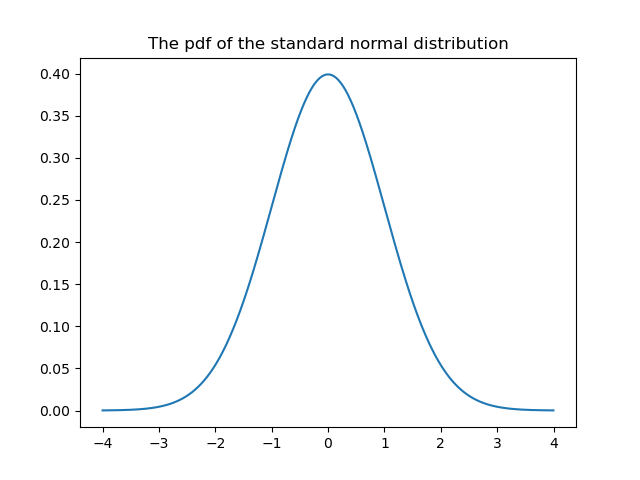
We can observe that the function we plotted above is an even function, i.e. $f(z)=f(-z)$ and its center is 0. Its inflection points are $-/+1$.
Let’s understand the purpose of each term of the expression. First we observe that the function \(\eqref{eq:eq1}\) is a product of a constant $\frac{1}{\sqrt{2\pi}}$ and a function of $z$, namely $\exp(\frac{-z^2}{2})$. The constant $\frac{1}{\sqrt{2\pi}}$ is called a normalizing constant. Its purpose is to make the integral of the function (the integral of a probability density function, is called its cumulative distribution function, cdf) equal 1. So the normalizing constant makes the function a probabilty density function. (Note, that this means that: $\int_{-\infty}^{\infty}{e^{-\frac{z}{2}^2}}dz = \sqrt{2\pi}$. A proof for this is given for example in Blitzstein and Hwang’s book “Introduction to Probability” on page 235.)
The expression $e^{(\frac{-z^2}{2})}$ is easy to understand:
- Squaring $z$ makes the function an even function, a parabola.
- The $-$ sign makes the parabola open downwards.
- Using $e$ as basis is very handy for doing derivatives of the function (if you don’t believe this, compute the first 3 derivatives of ${2}^{-z^2}$ and compare this to computing the first 3 derivatives of ${e}^{-z^2}$).
- The last question is why do we divide ${-z}^{2}$ by 2? The answer is that we want the inflection points of the pdf for the SND to be at $-1$ and $+1$. If we use ${-z}^{2}$ without dividing by 2, the inflection points are at $+/-\sqrt(1/2)$. Turns out, that dividing the expression by 2 is what we need to make the inflection points to be $-1$ and $1$.
Now we have a good understanding of the formula for the standard normal distribution. Now, let’s go a step further and think about what we need to do to shift this function to the left or to the right, thus horizontally. (If you need a refresher on this, google shifting and scaling functions, or look here, for a concise summary). We can subtract or add a constant to the independent variable, here $z$. If we want to scale a function we can multipy the variable $z$ by a constant. Let’s try this out: We want to shift the graph of the normal distribution two places to the right, so we need to subtract 2 from $z$. We also want to make it bigger by 3, so we divide $z$ by 3. The formula then is:
\[\begin{equation}f(z)=\frac{1}{\sqrt{2\pi}} * \exp(\frac{-\frac{(z – 2)}{3}^2}{2}), \quad -\infty<z<\infty\end{equation} \tag{1}\label{eq:eq2} \]
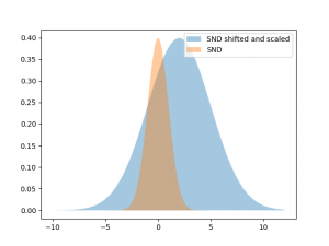
Let’s plot this:
As you can see, I plotted the graph of the pdf of the standard normal distribution for comparison. I also shaded the area underneath both graphs. The area underneath the pdf of the SND (its integral) equals $1$. We know that, because we just realized, that that’s the purpose of the factor $\frac{1}{\sqrt{2\pi}}$. We can see that the scaled and shifted version covers more area than our original SND. Thus its integral must be larger $1$, which means it is not a valid probability density function anymore. To fix this we need to divide it by an appropriate factor to make the integral $1$ again. This factor is just the value that we used to scale the graph, i.e. 3. To see this we do the following: We compute the area under the scaled and shifted graph and then we divide it by $3$ and compute the area again. We can do this in Python:
from sklearn.metrics import auc
import numpy as np

x = np.arange(-10, 12, 0.001)
dx = 0.001
y_shifted_scaled = 1/(np.power(2*np.pi,1/2))*np.exp((-1/2)*np.power((x-2)/3,2))
area_under_curve = auc(x,y_shifted_scaled)
print(area_under_curve)

y_shifted_scaled_normalized = 1/(np.power(2*np.pi,1/2)*3)*np.exp((-1/2)*np.power((x-2)/3,2))
area_under_curve_normalized = auc(x,y_shifted_scaled_normalized)
print(area_under_curve_normalized)
area_under_curve = 2.998616261980967
area_under_curve_normalized = 0.9995387539936558
So, the area under the shifted and scaled SND was 3 and dividing it by 3 made it 1. Wow! :). Thus, if we want the center of our parabola to be at a certain point, we just shift it to that point by subtracting a constant. Let’s call this constant $\mu$. If we want to scale it, we divide it by a constant. Let’s call this constant $\sigma$. Since dividing the variable by a constant makes it bigger (for a constant > 0 ), we can bring its integral back to one, if we divide the entire function by that constant. Thus, here we divide by $\sigma$. Let’s put this together, and instead of writing $exp()$ to denote the exponential function, we write $e^x$.
\[\begin{equation}f(x)=\frac{1}{\sqrt{2\pi} \sigma} e^{(\frac{-1}{2} (\frac{x – \mu}{\sigma})^2)}, \quad -\infty<x<\infty\end{equation} \tag{1}\label{eq:eq3} \]
Et voilá, we have the function for the normal distribution! Note, only ‘normal distribution’, no ‘standard’ in front. Also note that I replaced $z$ with $x$, since $z$ is usually used for the SND. So the normal distribution is a shifted, scaled and renormalized version of the standard normal distribution. Or in other words, the pdf of the standard normal distribution is a special case of the pdf of the normal distribution where $\mu = 0$ and $\sigma = 1$.
The pdf of the normal distribution is governed by $\mu$ and $\sigma$ that means the center of the graph is $\mu$ and the inflection points are at $\mu +/- \sigma$.
This post has also been published at medium.