The complete, friendly deep-dive into the core linear algebra every Data Scientist needs.

1 Introduction
Have you ever wondered how to unlock the secrets hidden in data but felt overwhelmed by the math? This article provides a friendly introduction to eigenvalues and eigenvectors which is a crucial linear algepra topic as it serves as the foundation for more advanced methods in data science, artificial intelligence, and machine learning. For example it is needed for understanding Singular Value Decomposition (SVD) and Principal Component Analysis (PCA).
Instead of just gaining intuition, we’ll explore both — core concepts and relevant math straightforwardly. Therefore, this guide will be valuable for beginners and professionals who seek to refresh their knowledge. By the end of this article, you’ll not only understand the significance of eigenvalues, eigenvectors, and matrix diagonalization, but also feel confident in applying these concepts to real-world problems.
2 Eigenvectors and Eigenvalues
One way to interpret eigenvectors is as distinct properties of a matrix. To understand this concept, let’s first set aside matrices. Consider a single number (a scalar): you could describe this number as even, greater than zero, or factorizable into specific components. It’s akin to filling out a friendship book for that number. You can apply this same approach to matrices. A matrix can be characterized by its size, determinant, rank, and, importantly, its eigenvectors and eigenvalues. So, what exactly is an eigenvector?
An eigenvector of a matrix A is a vector x, that when multiplied by the matrix, remains aligned along the same direction, though its magnitude may change. (see [2] p.289)
This concept is illustrated in Figure 2.

3 Formal Definition of an Eigenvector and Eigenvalue and Eigenvalues
We can formally define an eigenvector and eigenvalue as follows:

where:
- A ∈ ℝᵐˣⁿ is the matrix.
- x ∈ ℝⁿ is the eigenvector
- λ is a scalar (number) called the eigenvalue of A.
The interpretation of the eigenvalue is crucial:
- If λ > 1, the eigenvector is stretched;
- If 0 < λ < 1, the eigenvector is shrunk;
- If λ < 0, the eigenvector is reversed;
In Figure 2, entry d) illustrates the case of a negative eigenvalue. An eigenvalue can also be zero, which indicates that the according eigenvector lies in the null space of matrix A. This means that when A multiplies this vector, the result is the null vector.
In summary, if we have a vector x and a scalar λ for which the equation Ax = λx holds, we refer to x as an eigenvector and λ as the corresponding eigenvalue of A.
4 How to Compute the Eigenvectors and Eigenvalues of a Matrix?
To understand how to compute the eigenvectors and eigenvalues of a matrix A, we start by manipulating the eigenvector equation Ax = λx: This can be rewritten as:

Here, I denotes the identity matrix, which is a square matrix that has all zero entries except for ones on the diagonal. The identity matrix I must be of the same dimensions as A, meaning A must also be a square matrix. This is crucial, as it limits this method to square matrices! In line 3 we exploit the fact that (λI)x = λx. In line 4 we factor out x. The term in brackets (A − λI) is a matrix we denote as B which has n columns referred to as bᵢ . Thus, we have Bx = 0.
A matrix multiplied by a vector can equal the zero vector only if the matrix contains linear dependent columns. To illustrate this, we can rewrite the equation as follows:

From this representation, it is clear that a column of the matrix can be expressed as a linear combination of the other columns, which defines linear dependence. When a matrix exhibits linear dependence, we refer to it as singular. A singular matrix has a determinant of 0; for a proof see [2] p. 251.
This condition implies that for the equation in line 4 to hold, the determinant of (A − λI) must also be equal to 0. We express this as:

Here, det refers to the determinant. Equation 7 is fundamental for computing eigenvalues and eigenvectors; it is also known as the characteristic equation. This equation must be solved to determine the eigenvalues of a matrix. Once the eigenvalues are computed, you can substitute them back into the equation (A − λI)x = 0 to find the corresponding eigenvectors.
When solving this equation (a numerical example is provided in section 7) we will obtain a polynomial in λ of degree n, where n is the number of columns in A. Consequently, we may find up to n different solutions for λ: λ₁ , λ₂ , …λₙ . Thus, a matrix with n columns can have a maximum of n different eigenvalues.
For each eigenvalue λᵢ , we solve (A−λᵢ I)x = 0 to find the corresponding eigenvector. There is always at least one eigenvector associated with an eigenvalue since every multiple of that eigenvector will also be a solution to (A − λᵢ I)x. Because of this property, eigenvectors are typically normalized. We will see an example of how to compute eigenvalues and eigenvectors in section 7. For each eigenvalue we can solve (A − λᵢ I)x=0 to find the corresponding eigenvector.
It’s important to note that different λᵢ may have the same value; this phenomenon is referred to as the algebraic multiplicity of that eigenvalue. Now, let’s discuss a crucial piece of information in the next chapter
5 The Eigenbasis
When the algebraic multiplicity of all eigenvalues of a matrix is 1, it indicates that there are no repeated eigenvalues (all λᵢ are different).
In this case, all eigenvectors associated with these eigenvalues are linearly independent!
This – the linear independence- is a a very important point because it allows us to find as many linearly independent eigenvectors as there are columns in the matrix.
Thus, if A has no repeated eigenvalues, we can compute a full set of eigenvectors for it and stack those eigenvectors in a matrix. We know that they are linearly independent. This eigenvector matrix is a basis for A’s eigenspace. It is called A‘s eigenbasis. The eigenspace of a matrix consists of all the vectors it can legally be multiplied with and a basis is a set of linearly independent vectors in a vector space that spans the entire space, meaning any vector in that space can be expressed as a linear combination of the basis vectors. This process is known as the eigendecomposition of a matrix. The collection of eigenvalues is referred to as its spectrum of the matrix.
Again — if there are n distinct eigenvalues, we can compute n linearly independent eigenvectors, one for each eigenvalue. (Though every multiple of an eigenvector is also an eigenvector, we normalize it and treat it as one distinct vector.)
As a side note, it is indeed possible for the same eigenvalue to have more than one linearly independent eigenvector, but this only occurs when the algebraic multiplicity is greater than 1. For instance, an eigenvalue that appears twice can have up to two linearly independent eigenvectors associated with it. The number of linearly independent eigenvectors linked to an eigenvalue is always less than or equal to its algebraic multiplicity; this is known as the geometric multiplicity of that eigenvalue. A proof can be found here or see chapter 1 of [1] for more information).
6 Proof of Linearly Independent Eigenvectors for Different Eigenvalues
For a complete proof, refer to Strang’s text on page 306 [2]. Feel free to skip this subsection if it feels too detailed. However, for those readers seeking a detailed explanation rather than a mere assertion, I will present Strang’s proof specifically for a 2×2 matrix A.
Claim: I a matrix A ∈ ℝ²ˣ² has n different eigenvalues, then it has n linearly independent eigenvectors.
Assume we have computed two distinct eigenvalues λ₁ and λ₂ for A. We also have their normalized eigenvectors x₁ and x₂ . Our subjective is to demonstrate that these two eigenvectors are linearly independent.
The proof proceeds as follows: We start by assuming linear dependence (not independence) and will show that this leads to a contradiction. Consequently, the opposite must be true, i.e. the eigenvectors must must be linearly independent.
Two vectors are linearly dependent if there is a linear combination that gives the zero vector. Therefore, for some constants c₁ , and c₂ we can write:

If the zero vector can only be obtained by the trivial solution, where both coefficients are zero, then the vectors x₁ and x₂ are linearly independent. Next, we can multiply both sides of the equation 8 by the matrix A, using the fact that Axᵢ = λᵢ xᵢ .

Then multiply equation 8 by λ₂ to obtain:

We now have the equations 10 = 11:

We can substract c₂λ₂x₂ from both sides and move c₁λ₂x₂ to the left side. With this we obtain:

Factoring out c₁x₁ gives us:

But equation 15 can only hold true if either (λ₁− λ₂ ) = 0 or c₁x₁ = 0. Here are the conclusions:
- (λ₁ − λ2 ) = 0 implies that λ₁= λ₂. However, our initial assumption was that the eigenvalues are distinct, so this case cannot be true.
- c₁x₁ = 0 indicates that either c₁ = 0 or x₁ = 0. But eigenvectors cannot be zero vectors because if they were, the expression Ax = λx would hold for any λ and provide no meaningful information — we can discard this scenario.Thus, it follows that only c₁ can be 0.
Similary we can show that c₂ must also be zero.
If the linear combination c₁x₁ + c₂x₂ = 0 can only be true if the coefficients are zero, then we conclude that the vectors are linearly independent, by definition. Consequently, the opposite of our initial assumption (linear dependence) must be true: the eigenvectors are indeed linearly independent, as we aimed
to demonstrate.
7 A simple Example for Computing Eigenvalues and Eigenvectors
We will examine a simple example to compute the eigenvalues and eigenvectors of a 2×2 matrix A. Recall, that the determinant of a 2×2 matrix is given by the product of the upper left and lower right element minus the product of the upper right and lower left element. Assume:

To find the eigenvalues for A, we need to solve the equation det(A − λI). Thus, we have:

This simplifies to:

Calculating the determinant gives:

Now we can plug in the determinant into the equation 18 and obtain:

It’s important to note that the columns of A are linearly independent; that is, no column can be expressed as a multiple of the other. When we solve for the eigenvalues what we actually do is, we look for values that shift the matrix values such that A − λI becomes singular. In line 20, we obtain (2 − λ)² = 0. This is a second-order polynomial in λ (which can be expanded to 2² − 4λ + λ² ). As such it has two solutions, λ₁ and λ₂ . At a glance, we can see that the only value that makes (2 −−λ) zero is λ = 2 Therefore, we have an algebraic multiplicity of two, with λ₁ = λ₂ = 2.
The next step is to compute the eigenvectors corresponding to these eigenvalues. We do this by solving the equation (A − λI)x = 0. Substituting our value for λ:

This leads us to the following outcome:

From the first equation, we see that x₂ must be equal 0. There is no constraint on x₁, so it can take any value, t ∈ ℝ . We can express this relationship as follows:

Thus, any scalar multiple of [1, 0]ᵀ is an eigenvector associated with the eigenvalue 2.
We have just explored a simple example of how to compute the eigenvalues and eigenvectors of a matrix manually. For completeness, here is how you would do it in Python:
import numpy as np

# Define the matrix A
A = np.array([[2, 1],
              [0, 2]])

# Compute eigenvalues and eigenvectors
eigenvalues, eigenvectors = np.linalg.eig(A)

# Output results
print("Eigenvalues:", eigenvalues)
print("Eigenvectors:\n", eigenvectors)

#Eigenvalues: [2. 2.]
#Eigenvectors:
#[[ 1.0000000e+00 -1.0000000e+00]
#[ 0.0000000e+00  4.4408921e-16]]
Each column in the array ”eigenvectors” will contain an eigenvector, such as [1, 0]ᵀ and [−1, 0]ᵀ . These vectors lie on the same line and are consistent with our manually computed solution that the eigenvector is a scalar multiple of [1, 0]ᵀ . Note also that this matrix does not have a full set of distinct eigenvalues.
8 Summary of Key Points
The key points from the above discussion are:
- An eigenvector of a matrix A is a vector that remains on the same line after multiplication by A.
- There is always one eigenvalue for an eigenvector.
- There is at least one normalized eigenvector for a given eigenvalue.
- The eigenvalue acts like a scaling factor for the eigenvector.
- Eigenvalues are computed by solving det(A − λI) = 0, which is known as the characteristic equation of the matrix A. For each eigenvalue, we substitute its value into (A − λI) = 0, to obtain the associated normalized eigenvector x.
- There can be at most as many distinct eigenvalues as there are columns in A. However, some eigenvalues may repeat; which is referred to as the algebraic multiplicity of an eigenvalue.
- When there are no repeated eigenvalues (i.e. all λᵢ are distinct), it is guaranteed that there are as many linearly independent corresponding eigenvectors. In this case, there is one unique eigenvector associated to each eigenvalue. This linear independence enables a valid eigendecomposition of the matrix.
- All the above holds true only for square matrices.
9 References
[1] C. Johnson R. Horn. Matrix Analysis. Cambridge University Press, 2013. isbn: 9780521839402.
[2] Gilbert Strang. Introduction to Linear Algebra, Fifth Edition. Wellesley-Cambridge Press, 2016.
get a pdf:
Discover more from Master the Math
Subscribe to get the latest posts sent to your email.