Your Friendly Guide to the Math behind Data Science and AI

1 Introduction
Matrix diagonalization is a crucial concept in linear algebra with tons of applications. Even more importantly, it is the KEY to understanding advanced and essential data science topics like the singular value decomposition (SVD) and principal component analysis (PCA).
This article goes beyond intuition building only — it provides you with an accessible mathematical derivation of the topic, making it perfectly suitable for beginners while also serving as a knowledge refresher for seasoned professionals. It is meant as your friendly math guide.
So what is matrix diagonalization all about? It allows us to rewrite a matrix A in a simpler form involving a diagonal matrixD . This simplified form makes many otherwise difficult computations — like raising a matrix to a high power — trivial. Understanding matrix diagonalization is not difficult per se, but it builds on various other concepts, which will be presented in this text, however briefly. If you seek a deeper and more thorough understanding, you may want to refer to these articles on
There is also a pdf available at the end of this document with better math typesetting.
2 Deriving the Diagonalization Formula: AX = XΛ
In this section we will derive the fundamental matrix expression AX = XΛ which is the cornerstone of diagonalization. We start with the definition of an eigenvalue-eigenvector pair (x, λ) for a square matrix A:

This equation means that applying the transformation A to the vector x simply results in scaling x by the scalar λ, without changing its direction.
For an n × n matrix A we can potentially compute all the n eigenvalue-eigenvector pairs. We can then take all the eigenvectors x₁, x₂, . . . , xₙ, and stack them into a matrix, which we’ll call X (capital letter, to denote that its a matrix of vectors). For example, for
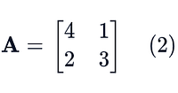
we can compute the two eigenvalue-eigenvector pairs λ₁ = 5, x₁ = [0.7, 0.7]ᵀ and λ₂ = 2, x₂ = [−0.4, 0.8]ᵀ . We can then form the matrix X by using these eigenvectors as its columns and we choose to start with the eigenvector that has the largest eigenvalue, x₁ and then we add the second eigenvector with the second-largest eigenvalue, x₂.

Next, we create a diagonal matrix, Λ (capital Lambda), which contains the corresponding eigenvalues on its main diagonal, in the exact same order as their eigenvectors in X:

While sorting the eigenvalues from largest to smallest, as we did here, is crucial in certain applications (like principal component analysis), the fundamental mathematical requirement is simply consistent ordering. That is, if you change the order of the columns in X (e.g., swapping x₁ and x₂), you must also swap the corresponding diagonal entries in Λ (i.e., λ₁ and λ₂ ) to maintain this correspondence.
With these definitions, the following fundamental expression is true — and we will show why:

(Note the order: it is XΛ, not the other way round.) To prove this identity, we will look at the result of the matrix multiplication on both sides of the equation and compare the columns.
2.1 The Left Side: AX
For the left side recall a key property of matrix multiplication: when a matrix X is multiplied by a matrix A, the resulting matrix’s columns are equal to A times the corresponding column of X (see here, for a refresher on matrix multiplication).

Now, we apply the definition of the eigenvalue-eigenvector pair, Ax = λx, to each column:

2.2 The Right Side: XΛ
For the right side, we use another fundamental property of matrix multiplication: multiplying a matrix X by a diagonal matrix Λ scales the columns of X by the corresponding diagonal elements of Λ. To see this, let’s look at the first column of the product XΛ for our n × n case:
The first column of Λ is the vector [ λ₁ , 0, . . . , 0]ᵀ. The multiplication X times this column gives:
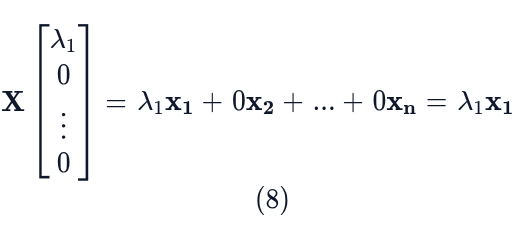
This process is repeated for every column of Λ. The i-th column of Λ is a vector with λᵢ in the i-th position and zeros elsewhere. Therefore, the i-th column of XΛ simplifies to λᵢxᵢ. Stacking these resulting columns gives us:
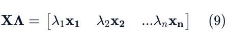
By comparing equation (7) and equation (9), we see that the columns of AX are identical to the columns of XΛ. Thus, it is clear that AX = XΛ is true.
3 Deriving the Diagonalization Formula: A = XΛX⁻¹
We established the fundamental matrix relationship AX = XΛ in the previous section. This expression is crucial for understanding matrix transformations and is the starting point for diagonalization. Now, let’s manipulate it further to isolate A and Λ. We start with this expression:
If, and only if, the matrix X is invertible (meaning X⁻¹ exists), we can post-multiply both sides by X⁻¹ to isolate A:

Alternatively, we can pre-multiply both sides of the original equation by X⁻¹ to isolate the diagonal matrix Λ:

3.1 When Can We Diagonalize? The Invertibility of X
This manipulation immediately raises a critical question: Can we always compute X⁻¹? The answer is no. The inverse X⁻¹ can only be computed when X is invertible. A matrix is invertible if and only if all of its columns (in this case, the eigenvectors x₁, x₂, . . . , xₙ ) are mutually linearly independent. A square n × n matrix is guaranteed to have n linearly independent eigenvectors if and only if for every eigenvalue, the geometric multiplicity equals the algebraic multiplicity, [Horn13] p. 77. (The algebraic multiplicity is the number of times an eigenvalue is a repeated root of the characteristic polynomial (e.g., λᵢ = λⱼ= 2). The geometric multiplicity is the number of linearly independent eigenvectors associated with that eigenvalue. We always have Geometric Multiplicity ≤ Algebraic Multiplicity
[strang˙16] p. 311.) A sufficient condition that guarantees this is if all of its n eigenvalues have distinct values (see here for more information or better a standard textbook on linear algebra). Therefore, the diagonalization formulae hold only for those special square matrices that possess n linearly independent eigenvectors.
3.2 A Geometrical Interpretation of Diagonalization
We have seen that if the conditions for X⁻¹ are met, we can rewrite the original matrix A as the product of three other matrices:

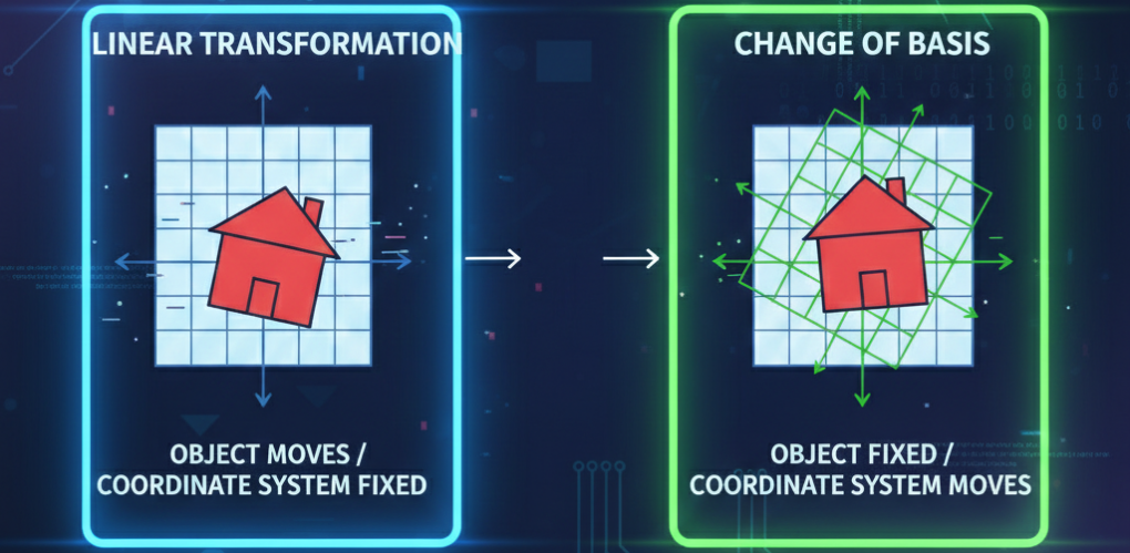
Since we have derived this formula we do have an abstract understanding of it, however, there is a very simple geometric interpretation, too and understanding this aspect in addition to the mathematical derivation will deepen our understanding of this process. Prerequisite is to have a solid understanding of linear transformations and change of basis as they work beautifully together in the process of diagonalization:
So here we go: We know that:
- D is a diagonal matrix. Diagonal matrices are highly desirable because they lead to greatly simplified computations (e.g., raising a matrix to a power).
- P is an invertible matrix whose columns are A’s eigenvectors. This matrix is also known as A’s eigenbasis.
- P⁻¹ is the inverse of the matrix of eigenvectors P.
Let’s say we apply A to some vector x. With diagonalization we can write this as:

And using the associativity of matrix multiplication we can compute this in the following order: (X(D(X⁻¹x))) We can see that this way diagonalization breaks the transformation down into three linked, simpler operations:
- (1) X⁻¹x: This is a change of basis. This means we transform the input vector x from the standard basis coordinates into the coordinates of A’s eigenbasis.

- (2) Dx_(eigenbasis): This is a simple transformation. We simply apply the diagonal matrix (D) to the new coordinates. Applying a diagonal matrix only involves a scaling of the components, making it computationally cheap.

- Xy_(eigenbasis): This is another change of basis. We use the original basis matrix (X) to transform the result back from the eigenbasis coordinates into our standard, familiar coordinate system.

In summary: Diagonalization can be interpreted as first transforming the input (x) into the matrix’s (A) eigenbasis. In this special representation the transformation reduces to a simple stretch of the input-vector into the various dimensions defined by the eigenvectors of A. And then we simply transform the result back into the standard basis.
4 Summary of Keypoints
Congratulations! Let’s review the crucial points that we’ve covered:
- We have derived the formula for matrix diagonalization to be A = XDX⁻¹.
- We know that at its core is A’s eigenbasis. If this can’t be computed, diagonalization with this method is not possible. You know that diagonalization is only possible for n × n square matrices where the following condition holds for every eigenvalue λ: Geometric Multiplicity of λ = Algebraic Multiplicity of λ. The simplest sufficient condition that guarantees this is for the matrix to have n distinct eigenvalues.
- Because of the above we understand the importance of eigenvalues and eigenvectors for matrix diagonalization.
- We understand that diagonalization has a geometric interpretation that involves expressing the input in terms of A’s eigenvectors, doing a then-simple stretch, and a transformation back into the standard basis.
While diagonalization is an excellent tool, its utility is limited to square matrices that have a complete and distinct set of eigenvalues.
So, where to go from here? Having established these fundamental concepts, the next major topic is the singular value decomposition (SVD). SVD represents a major leap forward in linear algebra. Essentially, SVD is a powerful generalization of diagonalization, enabling us to decompose any matrix—not just square ones. It is a more advanced, more general, and ultimately more versatile technique. But to understand SVD it was necessary to understand matrix diagonalization first.
References
[1] Roger A. Horn and Charles R. Johnson. Matrix Analysis. 2nd. Cambridge; New York: Cambridge University Press, 2013. isbn: 9780521839402.
[2] Gilbert Strang. Introduction to Linear Algebra, Fifth Edition. Wellesley-Cambridge
Press, 2016.
get a pdf:
Discover more from Master the Math
Subscribe to get the latest posts sent to your email.